A caixa de diálogo:guilabel:`Propriedades da camada ‘para uma camada vetorial fornece configurações gerais para gerenciar a aparência dos recursos da camada no mapa (simbologia, rotulagem, diagramas), interação com o mouse (ações, dicas de mapa, design de formulário). Ele também fornece informações sobre a camada.
Para acessar a caixa de diálogo:guilabel:Propriedades da camada:
No painel:guilabel:Camadas, clique duas vezes na camada ou clique com o botão direito do mouse e selecione: guilabel:` Propriedades… `no menu pop-up;
Vá para: seleção de menu: menu Camada -> Propriedades da camada … `quando a camada estiver selecionada.
O diálogo vetor:guilabel:Propriedades da camada fornece as seguintes seções:
** Compartilhe propriedades totais ou parciais dos estilos de camada **
A opção: seleção de menu: Estilo na parte inferior da caixa de diálogo permite importar ou exportar essas ou parte dessas propriedades de / para vários destinos (arquivo, área de transferência, banco de dados). Veja: ref: manage_custom_style.
Nota
Como as propriedades (simbologia, etiqueta, ações, valores padrão, formulários …) das camadas incorporadas (consulte:ref:` projetos de aninhamento`) são extraídas do arquivo original do projeto e, para evitar alterações que possam quebrar esse comportamento, o diálogo de propriedades da camada fica indisponível para essas camadas.
The Information tab is read-only and represents an interesting
place to quickly grab summarized information and metadata on the current layer.
Provided information are:
general such as name in the project, source path, list of auxiliary files,
last save time and size, the used provider
custom properties, used to store in the active project additional information about the layer.
Default custom properties may include layer notes,
legend widgets, layer variables,
form properties…
More custom properties can be created and managed using PyQGIS,
specifically through the setCustomProperty() method.
based on the provider of the layer: format of storage, geometry type,
data source encoding, extent, feature count…
o Sistema de Referência de Coordenadas: nome, unidades, método, precisão, referência (ou seja, se é estático ou dinâmico)
picked from the filled metadata: access, extents,
links, contacts, history…
e relacionados à sua geometria (extensão espacial, SRC…) ou seus atributos (número de campos, características de cada um…).
Set a Layer name different from the layer filename that will be
used to identify the layer in the project (in the Layers Panel, with
expressions, in print layout legend, …)
Depending on the data format, select the Data source encoding if not
correctly detected by QGIS.
Displays the layer’s Assigned Coordinate Reference System (CRS).
You can change the layer’s CRS, selecting a recently used one
in the drop-down list or clicking on Select CRS button
(see Seletor do Sistemas de Referência de Coordenadas). Use this process only if the CRS applied to the
layer is a wrong one or if none was applied.
If you wish to reproject your data into another CRS, rather use layer reprojection
algorithms from Processing or Save it into another layer.
Depending on the data provider, a Layer source group indicates the path
to the source of the dataset and allows for replacing the loaded layer:
When the layer is stored as file on disk, edit the path shown in the text box
or press …Browse to select another file on the disk.
Both layers do not need to share attribute fields, geometry type or file formats.
When the layer is provided by an ArcGIS Feature service,
it is possible to modify its authentication settings,
while keeping unchanged the details for connecting to the service.
Create spatial index (only for OGR-supported formats): helps speeding
layer rendering and features’ geometry retrieval.
:guilabel:informações da atualização de extensões para uma camada.
The Query Builder dialog is accessible through the Query Builder button
at the bottom of the Source tab in the Layer Properties dialog,
under the Provider feature filter group.
O Criador de consultas fornece uma interface que permite definir um subconjunto dos recursos na camada usando uma cláusula WHERE semelhante a SQL e exibir o resultado na janela principal. Enquanto a consulta estiver ativa, apenas os recursos correspondentes ao resultado estarão disponíveis no projeto.
You can use one or more layer attributes to define the filter in the QueryBuilder.
The use of more than one attribute is shown in Fig. 12.2.
In the example, the filter combines the attributes
Campo `` toa`` (`` Date Time``: `` cast (“toa” como personagem)>> 2017-05-17 ‘’) e `` cast (“toa” como personagem) <’2019-12 -24T18: 00: 00 ‘’),
usando os operadores AND, OR e NOT e parênteses. Essa sintaxe (incluindo o formato DateTime para o campo `` toa``) funciona para conjuntos de dados Pacote geográfico.
The filter is made at the data provider (OGR, PostgreSQL, MS SQL Server…) level.
So the syntax depends on the data provider (DateTime is for instance not
supported for the ESRI Shapefile format).
The complete expression:
Você também pode abrir a caixa de diálogo:guilabel:Criador de consultas usando a opção: guilabel:` Filtro … da opção: seleção de menus: menu Camada` ou menu contextual da camada. As seções:guilabel:` Campos`,: guilabel:` Valores` e:guilabel:Operadores na caixa de diálogo ajudam a construir a consulta semelhante a SQL exposta na caixa: guilabel:` Expressão de filtro específica do provedor`.
A lista ** Campos ** contém todos os campos da camada. Para adicionar uma coluna de atributo ao campo da cláusula SQL WHERE, clique duas vezes no nome ou digite-o na caixa SQL.
O quadro ** Valores ** lista os valores do campo selecionado no momento. Para listar todos os valores exclusivos de um campo, clique no botão: guilabel: Todos. Para listar os 25 primeiros valores exclusivos da coluna, clique no botão:guilabel:Amostra. Para adicionar um valor ao campo da cláusula SQL WHERE, clique duas vezes em seu nome na lista Valores. Você pode usar a caixa de pesquisa na parte superior do quadro Valores para navegar e encontrar facilmente os valores dos atributos na lista.
A seção ** Operadores ** contém todos os operadores utilizáveis. Para adicionar um operador ao campo da cláusula SQL WHERE, clique no botão apropriado. Operadores relacionais (`` = ,``>``,...),operadordecomparaçãodecadeias( LIKE``) e operadores lógicos (`` AND``, `` OR``, … ) Estão disponíveis.
The Test button helps you check your query and displays a message box with
the number of features satisfying the current query.
Use the Clear button to wipe the SQL query and revert the layer to its
original state (ie, fully load all the features).
It is possible to Save… the query as a .QQF file,
or Load… the query from a file into the dialog.
Quando um filtro é aplicado, o QGIS trata o subconjunto resultante como se fosse a camada inteira. Por exemplo, se você aplicou o filtro acima para ‘Bairro’ (`` “TYPE_2” = ‘Borough’),nãopoderáexibir,consultar,salvaroueditar``Ancoragem, porque é um’ Município ‘e portanto, não faz parte do subconjunto.
Dica
** As camadas filtradas são indicadas no painel Camadas **
In the Layers panel, filtered layer is listed with a Filter icon next to it indicating the query used when the mouse hovers over the button.
Double-click the icon opens the Query Builder dialog for edit.
This can also be achieved through the Layer ► Filter… menu.
The Symbology tab provides you with a comprehensive tool for
rendering and symbolizing your vector data. You can use tools that are
common to all vector data, as well as special symbolizing tools that were
designed for the different kinds of vector data. However all types share the
following dialog structure: in the upper part, you have a widget that helps
you prepare the classification and the symbol to use for features and at
the bottom the Renderização da camada widget.
Dica
** Alterne rapidamente entre diferentes representações de camada **
Usando a: seleção de menu: Estilos -> Add no final da caixa de diálogo: guilabel:Propriedades da camada, você pode salvar quantos estilos forem necessários. Um estilo é a combinação de todas as propriedades de uma camada (como simbologia, rotulagem, diagrama, formulário de campos, ações …) como você deseja. Em seguida, basta alternar entre os estilos no menu de contexto da camada em:guilabel:`Painel de camadas ‘para obter automaticamente diferentes representações dos seus dados.
Dica
Exportar simbologia vetorial
Você tem a opção de exportar a simbologia vetorial do QGIS para os arquivos das guias Google *. Kml, *. Dxf e MapInfo *. Basta abrir o menu direito do mouse da camada e clicar em: seleção de menu: Save As … para especificar o nome do arquivo de saída e seu formato. Na caixa de diálogo, use o menu: seleção de menu: Exportação de simbologia para salvar a simbologia como: seleção de menu:` Simbologia de recursos -> ou como: seleção de menu:
Simbologia da camada de símbolo -> `. Se você usou camadas de símbolos, é recomendável usar a segunda configuração.
The renderer is responsible for drawing a feature together with the correct
symbol. Regardless layer geometry type, there are four common types of
renderers: single symbol, categorized, graduated and rule-based. For point
layers, there are point displacement, point cluster and heatmap renderers available while
polygon layers can also be rendered with the merged features, inverted polygons and 2.5 D renderers.
Não há renderizador de cores contínuo, porque na verdade é apenas um caso especial do renderizador graduado. Os renderizadores classificados e graduados podem ser criados especificando um símbolo e uma rampa de cores - eles definirão as cores dos símbolos adequadamente. Para cada tipo de dados (pontos, linhas e polígonos), os tipos de camada de símbolo vetorial estão disponíveis. Dependendo do renderizador escolhido, a caixa de diálogo fornece diferentes seções adicionais.
Nota
Se você alterar o tipo de processador ao definir o estilo de uma camada de vetor as configurações feitas para o símbolo serão mantidas. Esteja ciente de que este procedimento só funciona para uma mudança. Se você repetir a alteração do tipo de renderizador as configurações para o símbolo irão se perder.
O | Símbolo único | :guilabel:o renderizador Símbolo único é usado para renderizar todos os recursos da camada usando um único símbolo definido pelo usuário. Veja:ref:`seletor de símbolos ‘para mais informações sobre representação de símbolos.
O | símbolo nulo | :guilabel:o renderizador Sem símbolos é um caso de uso especial do renderizador Símbolo único, pois aplica a mesma renderização a todos os recursos. Usando este renderizador, nenhum símbolo será desenhado para os recursos, mas ainda serão mostrados rótulos, diagramas e outras partes que não sejam de símbolos.
Ainda é possível fazer seleções na camada da tela e os recursos selecionados serão renderizados com um símbolo padrão. Os recursos editados também serão mostrados.
Este é um atalho útil para as camadas nas quais você deseja exibir apenas etiquetas ou diagramas e evita a necessidade de renderizar símbolos com preenchimento / borda totalmente transparente para conseguir isso.
O | símbolo categorizado | :guilabel:o renderizador categorizado é usado para renderizar os recursos de uma camada, usando um símbolo definido pelo usuário cujo aspecto reflete os valores discretos de um campo ou expressão.
Para usar a simbologia categorizada para uma camada:
Select the Value of classification: it can be an existing field
or an expression you can type in the box
or build using the associated button.
Using expressions for categorizing avoids the need to create a field for symbology purposes only
(eg, if your classification criteria are derived from one or more attributes).
A expressão usada para classificar recursos pode ser de qualquer tipo; por exemplo, pode:
seja uma comparação. Nesse caso, o QGIS retorna os valores `` 1`` (** True ) e `` 0`` ( False **). Alguns exemplos:
ser usado para transformar valores lineares em classes discretas, por exemplo:
CASEWHENx>1000THEN'Big'ELSE'Small'END
combine vários valores discretos em uma única categoria, por exemplo:
CASEWHENbuildingIN('residence','mobile home')THEN'residential'WHENbuildingIN('commercial','industrial')THEN'Commercial and Industrial'END
Dica
Embora você possa usar qualquer tipo de expressão para categorizar recursos, para algumas expressões complexas, pode ser mais simples usar:ref:renderização baseada em regras<rule_based_rendering>.
Configure o:ref:’Símbolol<symbol-selector>`, que será usado como símbolo base para todas as classes;
Indicate the Color ramp, i.e. the range of colors from which
the color applied to each symbol is selected.
Além das opções comuns do:ref:ferramenta de rampa de cores<color_ramp_widget>, você pode aplicar um | desmarcado | Random Color Ramp para as categorias. Você pode clicar na entrada: guilabel: Aleatório cores aleatórias para gerar novamente um novo conjunto de cores aleatórias, se você não estiver satisfeito.
Em seguida, clique no botão:guilabel:Classificar para criar classes a partir dos valores distintos do campo ou expressão fornecido.
For each class, you can edit the Legend column
to a more meaningful label (used in the Layers panel and the print layout).
Nota
Keep in mind that some values may use widgets that
do not display the actual value stored in the field.
For example, a checkbox widget may store 1 and 0 for checked and unchecked
states, while displaying True and False labels. In this case,
to categorize features based on the checkbox state, you need to use
the stored values (1 and 0) in the expression.
QGIS will automatically use the display value for the legend column.
Aplique as alterações se o: ref: atualização ao vivo <layer_styling_panel>`não estiver em uso e cada recurso na tela do mapa for renderizado com o símbolo de sua classe.
Por padrão, o QGIS anexa uma classe:guilabel:todos os outros valores à lista. Enquanto vazia no início, essa classe é usada como uma classe padrão para qualquer recurso que não se enquadre nas outras classes (por exemplo, quando você cria recursos com novos valores para o campo / expressão de classificação).
Outros ajustes podem ser feitos na classificação padrão:
You can Add new categories, Remove
selected categories, Delete All of them or Delete Unused categories.
Uma classe pode ser desativada desmarcando a caixa de seleção à esquerda do nome da classe; os recursos correspondentes estão ocultos no mapa.
Arraste e solte as linhas para reordenar as classes
Para alterar o símbolo, o valor ou a legenda de uma classe, clique duas vezes no item.
Clicar com o botão direito do mouse sobre os item (s) selecionados mostra um menu contextual para:
Copiar símbolo e: guilabel:` Colar símbolo`, uma maneira conveniente de aplicar a representação do item a outras pessoas
Alterar Color … do símbolo (s) selecionado
Alterar opacidade … do símbolo (s) selecionado
Alterar unidade de saída … do símbolo (s) selecionado
Alterar largura … do símbolo (s) de linha selecionado
Alterar tamanho … do símbolo (s) de ponto selecionado
Alterar ângulo … do símbolo (s) de ponto selecionado
Mesclar categorias: agrupa várias categorias selecionadas em uma única. Isso permite um estilo mais simples de camadas com um grande número de categorias, onde pode ser possível agrupar várias categorias distintas em um conjunto menor e mais gerenciável de categorias que se aplicam a vários valores.
Dica
Como o símbolo mantido para as categorias mescladas é o da categoria selecionada mais no topo da lista, convém mover a categoria cujo símbolo você deseja reutilizar para o topo antes de mesclar.
Unmerge Categories que foram mescladas anteriormente
The created classes also appear in a tree hierarchy in the Layers panel.
Double-click an entry in the map legend to edit the assigned symbol.
Right-click and you will get some more options.
O menu:guilabel:Avançado dá acesso a opções para acelerar a classificação ou ajustar a renderização de símbolos:
Corresponde aos símbolos salvos: Usando a: ref:` biblioteca de símbolos <vector_style_manager>`, atribui a cada categoria um símbolo cujo nome representa o valor de classificação da categoria
Corresponde aos símbolos do arquivo …: Fornece um arquivo com símbolos, atribui a cada categoria um símbolo cujo nome representa o valor de classificação da categoria
O símbolo | graduado | :guilabel:o renderizador Graduado é usado para renderizar todos os recursos de uma camada, usando um símbolo definido pelo usuário cuja cor ou tamanho reflete a atribuição do atributo de um recurso selecionado a uma classe.
Como o Renderizador categorizado, o Renderizador graduado permite definir a rotação e a escala de tamanho das colunas especificadas.
Além disso, de forma análoga ao Renderizador Categorizado, permite selecionar:
The Value of classification: it can be an existing field
or an expression you can type in the box
or build using the associated button.
Using expressions for graduating avoids the need to create a field for symbology purposes only
(eg, if your classification criteria are derived from one or more attributes).
O símbolo (usando a caixa de diálogo Seletor de símbolos)
O formato da legenda e a precisão
O método a ser usado para alterar o símbolo: cor ou tamanho
As cores (usando a lista Rampa de cores) se o método de cores estiver selecionado
O tamanho (usando o domínio de tamanho e sua unidade)
Em seguida, você pode usar a guia Histograma, que mostra um histograma interativo dos valores do campo ou expressão atribuído. As quebras de classe podem ser movidas ou adicionadas usando o widget de histograma.
Nota
Você pode usar o painel Resumo Estatístico para obter mais informações sobre sua camada vetorial. Veja:ref:”resumo estatístico”.
De volta à guia Classes, você pode especificar o número de classes e também o modo para classificar os recursos dentro das classes (usando a lista Modo). Os modos disponíveis são:
Equal Count (Quantile): each class will have the same number of elements
(the idea of a boxplot).
Intervalo igual: cada classe terá o mesmo tamanho (por exemplo, com os valores de 1 a 16 e quatro classes, cada classe terá um tamanho de quatro).
Fixed Interval: each class will have a fixed range of values (e.g. with the
values from 1 to 16 and an interval size of 4, the classes will be 1-4,
5-8, 9-12 and 13-16).
Logarithmic scale: suitable for data with a wide range of values.
Narrow classes for low values and wide classes for large values (e.g. for
decimal numbers with range [0..100] and two classes, the first class will
be from 0 to 10 and the second class from 10 to 100).
Natural Breaks (Jenks): the variance within each class is minimized while
the variance between classes is maximized.
Pretty Breaks: computes a sequence of about n+1 equally spaced nice values
which cover the range of the values in x. The values are chosen so that they
are 1, 2 or 5 times a power of 10. (based on pretty from the R statistical
environment https://www.rdocumentation.org/packages/base/topics/pretty).
Desvio padrão: as classes são construídas dependendo do desvio padrão dos valores.
A caixa de listagem na parte central da guia:guilabel:Simbologia lista as classes, juntamente com seus intervalos, rótulos e símbolos que serão renderizados.
Clique no botão ** Classificar ** para criar classes usando o modo escolhido. Cada classe pode ser desativada desmarcando a caixa de seleção à esquerda do nome da classe.
Para alterar o símbolo, valor e/ou rótulo da classe, basta clicar duas vezes no item que você deseja alterar.
Clicar com o botão direito do mouse sobre os item (s) selecionados mostra um menu contextual para:
Copiar símbolo e: guilabel:` Colar símbolo`, uma maneira conveniente de aplicar a representação do item a outras pessoas
Alterar Color … do símbolo (s) selecionado
Alterar opacidade … do símbolo (s) selecionado
Alterar unidade de saída … do símbolo (s) selecionado
Alterar largura … do símbolo (s) de linha selecionado
Alterar tamanho … do símbolo (s) de ponto selecionado
Alterar ângulo … do símbolo (s) de ponto selecionado
The example in Fig. 12.5 shows the graduated rendering dialog for
the major_rivers layer of the QGIS sample dataset.
The created classes also appear in a tree hierarchy in the Layers panel.
Double-click an entry in the map legend to edit the assigned symbol.
Right-click and you will get some more options.
Símbolo proporcional e análise multivariada não são tipos de renderização disponíveis na lista suspensa Renderização de simbologia. No entanto, com as opções:ref:substituição definida por dados<data_defined> aplicada a qualquer uma das opções de renderização anteriores, o QGIS permite exibir seus dados de ponto e linha com essa representação.
** Criando símbolo proporcional **
Para aplicar uma renderização proporcional:
Primeiro aplique à camada o:ref:renderizador de símbolo único<single_symbol_renderer>.
Em seguida, defina o símbolo para aplicar aos recursos.
Selecione o item no nível superior da árvore de símbolos e use o | dadosDefinidos | Substituição definida por dados: ref:` botão<data_defined> ao lado da opção: guilabel:`Tamanho (para camada de pontos) ou:guilabel:Largura (para camada de linha).
Selecione um campo ou insira uma expressão e, para cada recurso, o QGIS aplicará o valor de saída à propriedade e redimensionará proporcionalmente o símbolo na tela do mapa.
Se necessário, use a opção:guilabel:Assistente de tamanho … da | dadosDefinidos | menu para aplicar alguma transformação (exponencial, flannery …) ao redimensionamento do tamanho do símbolo (consulte:ref:assistente_dados_definidos para obter mais detalhes).
Você pode optar por exibir os símbolos proporcionais na:ref:Camadas do painel e na: ref:` item da legenda do layout de impressão : desdobre a lista suspensa: guilabel: Avançado` na parte inferior da caixa de diálogo principal do :guilabel:aba Simbologia e selecione ** Legenda do tamanho definido pelos dados … ** para configurar os itens da legenda (consulte: ref:` legenda_tamanho_multado _dados` para obter detalhes).
** Criando análise multivariada **
Uma renderização de análise multivariada ajuda a avaliar o relacionamento entre duas ou mais variáveis, por exemplo, uma pode ser representada por uma rampa de cores enquanto a outra é representada por um tamanho.
A maneira mais simples de criar análises multivariadas no QGIS é:
Primeiro, aplique uma renderização categorizada ou graduada em uma camada, usando o mesmo tipo de símbolo para todas as classes.
Em seguida, aplique uma simbologia proporcional nas classes:
Clique no botão:guilabel:Mudança acima do quadro de classificação: você obtém a caixa de diálogo: ref:` seletor de símbolos`.
Como o símbolo proporcional, a simbologia escalada pode ser adicionada à árvore de camadas, sobre os símbolos das classes categorizadas ou graduadas, usando o recurso:ref:legenda do tamanho definido dos dados<data_defined_size_legend>. E ambas as representações também estão disponíveis no item da legenda do layout de impressão.
Fig. 12.6 Exemplo multivariado com legenda de tamanho dimensionado
Rules are QGIS expressions used to discriminate
features according to their attributes or properties in order to apply specific
rendering settings to them. Rules can be nested, and features belong to a class
if they belong to all the upper nesting level(s).
The Rule-based renderer is thus designed
to render all the features from a layer, using symbols whose aspect
reflects the assignment of a selected feature to a fine-grained class.
Para criar uma regra:
Activate an existing row by double-clicking it (by default, QGIS adds a
symbol without a rule when the rendering mode is enabled) or click the
Edit rule or Add rule button.
Na caixa de diálogo:guilabel:Editar regra que é aberta, você pode definir um rótulo para ajudá-lo a identificar cada regra. Este é o rótulo que será exibido em:guilabel:`Painel de camadas ‘e também na legenda do compositor de impressão.
Insira manualmente uma expressão na caixa de texto ao lado de | botão de opção Ativado | :guilabel:opção Filtro ou pressione a expressão | ao lado dele para abrir a caixa de diálogo do construtor de cadeias de expressão.
Use as funções fornecidas e os atributos da camada para criar uma expressão: ref:<vector_expressions> para filtrar os recursos que você deseja recuperar. Pressione o botão:guilabel:`Test para verificar o resultado da consulta.
Você pode inserir um rótulo mais longo para concluir a descrição da regra.
Você pode usar a caixa de seleção | :guilabel:opção ` Escala de escala` para definir escalas nas quais a regra deve ser aplicada.
Por fim, configure o símbolo:ref:para usar<symbol-selector> para esses recursos.
E pressione:guilabel:OK.
Uma nova linha que resume a regra é adicionada à caixa de diálogo Propriedades da camada. Você pode criar quantas regras forem necessárias, seguindo as etapas acima ou copiar colando uma regra existente. Arraste e solte as regras uma sobre a outra para aninhar e refinar os recursos da regra superior nas subclasses.
The rule-based renderer can be combined with categorized or graduated renderers.
Selecting a rule, you can organize its features in subclasses using the
Refine selected rules drop-down menu. Refined classes appear like
sub-items of the rule, in a tree hierarchy and like their parent, you can set
the symbology and the rule of each class.
Automated rule refinement can be based on:
scales: given a list of scales, this option creates a set of classes
to which the different user-defined scale ranges apply. Each new scale-based
class can have its own symbology and expression of definition.
This can e.g. be a convenient way to display the same features with various
symbols at different scales, or display only a set of features depending on
the scale (e.g. local airports at large scale vs international airports at
small scale).
categories: applies a categorized renderer
to the features falling in the selected rule.
or ranges: applies a graduated renderer
to the features falling in the selected rule.
Refined classes appear like sub-items of the rule, in a tree hierarchy and like
above, you can set symbology of each class.
Symbols of the nested rules are stacked on top of each other so be careful in
choosing them. It is also possible to uncheck Symbols
in the Edit rule dialog to avoid rendering a particular symbol
in the stack.
Na caixa de diálogo:guilabel:Editar regra, você pode evitar escrever todas as regras e usar o | botão de rádio desativado | :guilabel:opção Outra para capturar todos os recursos que não correspondem a nenhuma das outras regras, no mesmo nível. Isso também pode ser conseguido escrevendo Outra na coluna * Rule * da seção: seleção de menus: Propriedades da camada -> Simbologia-> Baseado em regras.
Clicar com o botão direito do mouse sobre os item (s) selecionados mostra um menu contextual para:
Copiar e: guilabel:` Colar`, uma maneira conveniente de criar novos item com base nos itens existentes
Copiar símbolo e: guilabel:` Colar símbolo`, uma maneira conveniente de aplicar a representação do item a outras pessoas
Alterar Color … do símbolo (s) selecionado
Alterar opacidade … do símbolo (s) selecionado
Alterar unidade de saída … do símbolo (s) selecionado
Alterar largura … do símbolo (s) de linha selecionado
Alterar tamanho … do símbolo (s) de ponto selecionado
Alterar ângulo … do símbolo (s) de ponto selecionado
Refine Current Rule: open a submenu that allows to
refine the current rule with scales, categories or Ranges.
Same as selecting the corresponding menu
at the bottom of the dialog.
Unchecking a row in the rule-based renderer dialog hides in the map canvas
the features of the specific rule and the nested ones.
The created rules also appear in a tree hierarchy in the map legend.
Double-click an entry in the map legend to edit the assigned symbol.
Right-click and you will get some more options.
The example in Fig. 12.7 shows the rule-based rendering
dialog for the rivers layer of the QGIS sample dataset.
Fig. 12.7 Opções de simbolização baseadas em regras
The Point Displacement renderer takes
the point features falling in a given distance tolerance from each other and
places their symbols around their barycenter, following different placement
methods. This can be a convenient way to visualize all the features of a point
layer, even if they have the same location (e.g. amenities in a building).
To configure a point displacement renderer, you have to:
Set the Center symbol: how the virtual point at the center will
look like
Select the Renderer type: how you want to classify features
in the layer (single, categorized, rule-based…)
Press the Renderer Settings… button to configure features’
symbology according to the selected renderer
Indicate the Distance tolerance in which close features are
considered overlapping and then displaced over the same virtual point.
Supports common symbol units.
Configure the Placement methods:
** Toque **: coloca todos os recursos em um círculo cujo raio depende do número de recursos a serem exibidos.
** Anéis concêntricos **: usa um conjunto de círculos concêntricos para mostrar os recursos.
** Grade **: gera uma grade regular com um símbolo de ponto em cada interseção.
Displaced symbols are placed on the Displacement lines.
While the minimal spacing of the displacement lines depends on the
point symbols renderer, you can still customize some of their settings such as
the Stroke width, Stroke color and Size
adjustment (e.g., to add more spacing between the rendered points).
Use the Labels group options to perform points labeling: the labels
are placed near the displaced symbol, and not at the feature real position.
Select the Label attribute: a field of the layer to use for labeling
Indicate the Label font properties and size
Pick a Label color
Set a Label distance factor: for each point feature, offsets
the label from the symbol center proportionally to the symbol’s diagonal size.
Turn on Use scale dependent labeling
if you want to display labels only on scales larger than a given
Minimum map scale.
O renderizador de deslocamento de ponto não altera a geometria do recurso, o que significa que os pontos não são movidos de sua posição. Eles ainda estão localizados em seu local inicial. As alterações são apenas visuais, para fins de renderização. Em vez disso, use o algoritmo Em processamento: ref: qgispointsdisplacement se desejar criar recursos deslocados.
Unlike the Point Displacement renderer
which blows up nearest or overlaid point features placement, the Point Cluster renderer groups nearby points into a single
rendered marker symbol. Points that fall within a specified distance
from each others are merged into a single symbol.
Points aggregation is made based on the closest group being formed, rather
than just assigning them the first group within the search distance.
Na caixa de diálogo principal, você pode:
Set the symbol to represent the point cluster in the Cluster symbol;
the default rendering displays the number of aggregated features thanks to the
@cluster_sizevariable on Font marker
symbol layer.
Select the Renderer type, i.e. how you want to classify features
in the layer (single, categorized, rule-based…)
Press the Renderer Settings… button to configure features’ symbology
as usual. Note that this symbology is only visible on features that are not clustered,
the Cluster symbol being applied otherwise.
Also, when all the point features in a cluster belong to the same rendering class,
and thus would be applied the same color, that color represents the @cluster_color
variable of the cluster.
Indicate the maximal Distance to consider for clustering features.
Supports common symbol units.
O renderizador de cluster de pontos não altera a geometria do recurso, o que significa que os pontos não são movidos de sua posição. Eles ainda estão localizados em seu local inicial. As alterações são apenas visuais, para fins de renderização. Em vez disso, use o algoritmo em processamento:ref:qgiskmeansclustering ou: ref:` qgisdbscanclustering` se desejar criar recursos baseados em cluster.
The Merged Features renderer allows area and line
features to be “dissolved” into a single object prior to rendering to ensure that
complex symbols or overlapping features are represented by a uniform and
contiguous cartographic symbol.
O | símbolo invertido | :guilabel:O renderizador Polígono invertido permite ao usuário definir um símbolo a ser preenchido fora dos polígonos da camada. Como acima, você pode selecionar sub-remetentes, ou seja, renderizador de símbolo único, graduado, categorizado, baseado em regras ou 2.5D.
With the Heatmap renderer you can create live
dynamic heatmaps for (multi)point layers.
You can specify the heatmap Radius in millimeters, points, pixels, map units or
inches, choose and edit a Color ramp for the heatmap style and use a slider for
selecting a trade-off between render speed and quality. You can also define a
Maximum value limit and Weight points by using a field or an expression.
Use Data defined override to dynamically control Radius and
Maximum value based on the attributes of your data.
For example, the radius of a heatmap point could be determined by its population attribute,
or the maximum value could be based on a temporal range.
When adding or removing a feature the heatmap renderer updates the heatmap style
automatically. The Color ramp will be shown as a legend bar and
in the Legend settings you can set the Labels for the Maximum
and Minimum values. You can also change the orientation and direction of the legend
in the Layout.
Usando o | 25dSymbol | :guilabel:renderizador 2.5D é possível criar um efeito 2.5D nos recursos da sua camada. Você começa escolhendo um valor: guilabel: Altura (em unidades do mapa). Para isso, você pode usar um valor fixo, um dos campos da sua camada ou uma expressão. Você também precisa escolher um:guilabel:Ângulo (em graus) para recriar a posição do visualizador (0 | graus | significa oeste, crescendo no sentido anti-horário). Use opções de configuração avançadas para definir:guilabel:Cor do telhado e: guilabel:` Cor da parede`. Se você deseja simular radiação solar nas paredes dos recursos, marque a caixa de seleção | :guilabel:opção Paredes sombreadas com base no aspecto. Você também pode simular uma sombra definindo a:guilabel:Cor e: guilabel:` Size` (em unidades do mapa).
** Usando o efeito 2.5D com outros renderizadores **
Depois de concluir a configuração do estilo básico no renderizador 2.5D, você poderá convertê-lo em outro renderizador (único, categorizado e graduado). Os efeitos 2.5D serão mantidos e todas as outras opções específicas do renderizador estarão disponíveis para você ajustá-los (desta forma, você pode ter, por exemplo, símbolos categorizados com uma boa representação 2.5D ou adicionar um estilo extra aos seus símbolos 2.5D). Para garantir que a sombra e o “edifício” em si não interfiram com outros recursos próximos, pode ser necessário ativar os Níveis de símbolos (: menuelection: Advanced -> Symbol levels …). Os valores de altura e ângulo de 2.5D são salvos nas variáveis da camada, para que você possa editá-lo posteriormente na guia variáveis da caixa de diálogo de propriedades da camada.
The Embedded Symbols renderer allows to display the ‘native’
symbology of a provided datasource. This is mostly the case with KML
and TAB datasets that have predefined symbology.
Na guia da Simbologia, você também pode definir algumas opções que atuam invariavelmente em todos os recursos da camada:
Opacity: You can make the underlying layer in
the map canvas visible with this tool. Use the slider to adapt the visibility
of your vector layer to your needs. You can also make a precise definition of
the percentage of visibility in the menu beside the slider.
Blending mode at the Layer and Feature levels:
You can achieve special rendering effects with these tools that you may previously
only know from graphics programs. The pixels of your overlaying and
underlying layers are mixed through the settings described in Modos de Mistura.
Aplique:ref:efeitos de pintura<draw_effects> em todos os recursos da camada com o botão:guilabel: Efeitos de desenho.
Controlar a ordem de renderização do recurso ‘permite que você, usando atributos de recursos, defina a ordem z na qual eles serão renderizados. Ative a caixa de seleção e clique no | classificar | botão ao lado. Você então recebe a caixa de diálogo:guilabel:`Definir ordem na qual você:
Escolha um campo ou crie uma expressão para aplicar aos recursos da camada.
Defina em que ordem os recursos buscados devem ser classificados, ou seja, se você escolher a ordem ** Ascendente **, os recursos com valor mais baixo serão renderizados naqueles com valor mais alto.
Defina quando os recursos que retornam valor NULO devem ser renderizados: ** primeiro ** (inferior) ou ** último ** (superior).
Repita as etapas acima quantas vezes você desejar.
A primeira regra é aplicada a todos os recursos da camada, ordenando-os de acordo com o valor retornado. Em seguida, dentro de cada grupo de recursos com o mesmo valor (incluindo aqueles com valor NULO) e, portanto, o mesmo nível z, a próxima regra é aplicada para classificá-los. E assim por diante…
Para renderizadores que permitem camadas de símbolos empilhados (apenas o mapa de calor não), existe uma opção para controlar a ordem de renderização dos níveis de cada símbolo.
Para a maioria dos renderizadores, você pode acessar a opção Níveis de símbolos clicando no botão:guilabel:Avançado abaixo da lista de símbolos salvos e escolhendo: guilabel:` Níveis de símbolos`. Para o:ref:renderização baseada em regras, a opção está diretamente disponível através do botão:guilabel:Símbolos Níveis … `, enquanto para o renderizador ref:`deslocamento de ponto o mesmo botão está dentro da caixa de diálogo:guilabel:Configurações de renderização
Para ativar os níveis de símbolos, marque a caixa de seleção | Ativar níveis de símbolo. Cada linha exibirá uma pequena amostra do símbolo combinado, seu rótulo e a camada de símbolos individuais divididos em colunas com um número ao lado. Os números representam o nível da ordem de renderização no qual a camada de símbolo será desenhada. Os níveis de valores mais baixos são desenhados primeiro, permanecendo na parte inferior, enquanto os valores mais altos são desenhados por último, sobre os outros.
Se os níveis de símbolos estiverem desativados, os símbolos completos serão desenhados de acordo com a respectiva ordem de recursos. Símbolos sobrepostos simplesmente serão ofuscados para os outros abaixo. Além disso, símbolos semelhantes não “se fundem” entre si.
Fig. 12.15 Diferença nos níveis de símbolo ativado (A) e desativado (B)
Quando uma camada é renderizada com o símbolo:ref:proporcional ou multivariado<proportional_symbols> ou quando um:ref:diagrama de tamanho em escala<diagram_size> é aplicado à camada, você pode permitir a exibição dos símbolos em escala em ambos:ref:Camadas do painel<label_legend> e: ref: legenda do layout de impressão<layout_legend_item>.
Para ativar a caixa de diálogo:guilabel:Legenda do tamanho definido por dados para renderizar simbologia, selecione a opção de epônimo no botão: guilabel:` Avançado` abaixo da lista de símbolos salvos. Para diagramas, a opção está disponível na guia:guilabel:guia Legenda. A caixa de diálogo fornece as seguintes opções para:
selecione o tipo de legenda: | botão de opção Ativado | Legenda não ativada, | botão de opção Desativado | Itens de legenda separados e |botão de opção Desativado | legenda recolhida. Para a última opção, você pode selecionar se os itens da legenda estão alinhados na ** Parte inferior ** ou no ** Centro **;
preview the symbol to use for legend representation;
insira o título na legenda;
redimensionar as classes a serem usadas: por padrão, o QGIS fornece uma legenda de cinco classes (com base em pausas bonitas naturais), mas você pode aplicar sua própria classificação usando a caixa de seleção | : guilabel: opção Classes de tamanho manual. Use o | assinarPlus | e | assinar menos | para definir seus valores e rótulos de classes personalizadas.
For collapsed legend, it’s possible to:
Align symbols in the center or the bottom
configure the horizontal leader Line symbol from the symbol
to the corresponding legend text.
A preview of the legend is displayed in the right panel of the dialog and
updated as you set the parameters.
Fig. 12.16 Configurando legenda em tamanho dimensionado
Nota
Atualmente, a legenda do tamanho definido pelos dados para a simbologia de camada só pode ser aplicada à camada de ponto usando uma simbologia única, categorizada ou graduada.
To allow any symbol to become an animated symbol,
you can utilize Animation settings panel. In this panel,
you can enable animation for the symbol and set a specific frame rate for
the symbol’s redrawing.
Start by going to the top symbol level and select Advanced
menu in the bottom right of the dialog
Find Animation settings option
Check Is Animated to enable animation for the symbol
Configure the Frame rate, i.e. how fast the animation would
be played
You can now use @symbol_frame variable in any sub-symbol data defined
property in order to animate that property.
For example, setting the symbol’s rotation to data
defined expression @symbol_frame%360
will cause the symbol to rotate over time, with rotation speed dictated by
the symbol’s frame rate:
Fig. 12.17 Setting the symbol’s rotation to data defined expression
You may set an extent buffer for a symbol. This means that a buffer is applied to
the current map extent so that if a feature is outside of the actual map extent
but inside the buffered extent it will still be rendered. This is useful for example
with symbols which use the geometry generator where you would like to still see the
generated geometries even if the actual feature is outside of the map extent.
To edit the extent buffer you can utilize the Extent buffer panel.
Start by going to the top symbol level and select Advanced
menu in the bottom right of the dialog
Find Extent buffer option
In the new panel you can set the buffer distance
The buffer distance units can be changed. You can also control the distance value
by using the data defined override widget. For example you can change the value
based on the current map scale if(@map_scale>50000,5000,0):
Fig. 12.18 Example of the extent buffer with a symbol using a geometry generator symbol level.
Para melhorar a renderização da camada e evitar (ou pelo menos reduzir) o recurso a outro software para a renderização final dos mapas, o QGIS fornece outra funcionalidade poderosa: os | Efeitos de pintura | :guilabel:opções Efeitos de desenho, que adicionam efeitos de pintura para personalizar a visualização de camadas vetoriais.
A opção está disponível na caixa de diálogo: seleção de menus: Propriedades da camada-> Simbologia, no grupo: ref:` Renderização de camada <layer_rendering>`(aplicável a toda a camada) ou em: ref:` propriedades da camada de símbolo<symbol-selector> `(aplicável às correspondentes recursos). Você pode combinar os dois usos.
Paint effects can be activated by checking the Draw effects option
and clicking the Customize effects button. That will open
the Effect Properties Dialog (see Fig. 12.19). The following
effect types, with custom options are available:
** Origem **: desenha o estilo original do recurso de acordo com a configuração das propriedades da camada. O:guilabel:Opacidade do seu estilo pode ser ajustado assim como: ref:` Modo de mistura` e:ref:Modo Draw. Essas são propriedades comuns para todos os tipos de efeitos.
Fig. 12.19 Efeitos de desenho: caixa de diálogo Origem
** Desfoque **: adiciona um efeito de desfoque na camada vetorial. As opções personalizadas que você pode alterar são:guilabel:` Tipo de desfoque` (: guilabel:` Desfoque de pilha (fast) ou: guilabel: Desfoque Gaussiano (qualidade) ) e: guilabel:`Força do borrão.
Fig. 12.20 Efeitos de desenho: caixa de diálogo Blur
** Colorizar **: esse efeito pode ser usado para criar uma versão do estilo usando uma única tonalidade. A base sempre será uma versão em escala de cinza do símbolo e você pode:
Use o | selecione String | Escala de cinza para selecionar como criá-la: as opções são ‘Por luminosidade’, ‘Por luminosidade’, ‘Por média’ e ‘Desligado’.
Se | caixa de seleção | Colorise está selecionado, será possível misturar outra cor e escolher quão forte ela deve ser.
Controle os níveis:guilabel:Brilho,: guilabel:` Contraste` e:guilabel:Saturaturação do símbolo resultante.
Fig. 12.21 Efeitos de desenho: caixa de diálogo Colorir
** Sombra projetada **: o uso desse efeito adiciona uma sombra ao recurso, que parece adicionar uma dimensão extra. Este efeito pode ser personalizado alterando o:guilabel:ângulo e distância do ` Deslocamento ‘, determinando para onde a sombra se desloca e a proximidade do objeto de origem. : menuselection: Drop Shadow também tem a opção de alterar: guilabel:` Raio de desfoque` e:guilabel:Corr do efeito.
Fig. 12.22 Caixa de diálogo Efeitos de desenho: Sombra projetada
** Sombra interior**: Este efeito é semelhante ao efeito:guilabel:Drop Shadow, mas adiciona o efeito de sombra na parte interna das bordas do recurso. As opções disponíveis para personalização são as mesmas do efeito: guilabel: Sombra projetada.
Fig. 12.23 Caixa de diálogo Efeitos de desenho: Sombra interna
** Brilho interno **: adiciona um efeito de brilho dentro do recurso. Este efeito pode ser personalizado ajustando:guilabel:Espalhe (largura) do brilho ou: guilabel:` Raio de desfoque`. Este último especifica a proximidade da borda do recurso em que você deseja que ocorra qualquer desfoque. Além disso, existem opções para personalizar a cor do brilho usando a:guilabel:Única cor ou a: guilabel:` Rampa de cores`.
Fig. 12.24 Caixa de diálogo Efeitos de desenho: Brilho interno
** Brilho externo **: Este efeito é semelhante ao efeito:guilabel:Brilho interno, mas adiciona o efeito de brilho na parte externa das bordas do recurso. As opções disponíveis para personalização são as mesmas do efeito: guilabel: Brilho interior.
Fig. 12.25 Caixa de diálogo Draw Effects: Brilho externo
Transform: Adds the possibility of transforming the shape of the symbol.
The first options available for customization are the Reflect
horizontal and Reflect vertical, which actually create a
reflection on the horizontal and/or vertical axes. The other options are:
Shear X, Y: inclina o recurso ao longo do eixo X e / ou Y.
Escala X, Y: amplia ou minimiza o recurso ao longo do eixo X e / ou Y pela porcentagem especificada.
Rotação: gira o recurso em torno de seu ponto central.
e:guilabel:”Traduzir X, Y” altera a posição do item com base na distância indicada no eixo X e / ou Y.
Fig. 12.26 Caixa de diálogo Efeitos de desenho: transformação
Um ou mais tipos de efeito podem ser usados ao mesmo tempo. Você (des) ativa um efeito usando sua caixa de seleção na lista de efeitos. Você pode alterar o tipo de efeito selecionado usando o | selecione String | : guilabel: opção Tipo de efeito. Você pode reordenar os efeitos usando | seta para cima | Mover para cima e | seta para baixo | :sup:botões Mover para baixo e também adicionar / remover efeitos usando o | assinar mai | Adicionar novo efeito e | assinar menos | :sup:botões Remover efeito.
Existem algumas opções comuns disponíveis para todos os tipos de efeito de desenho. As opções:guilabel:Opacidade e: guilabel:` Modo de mistura` funcionam de maneira semelhante às descritas em:ref:renderização de camada e podem ser usadas em todos os efeitos de desenho, exceto o de transformação.
Há também uma |selecione String | :guilabel:opção `Draw mode ‘disponível para todos os efeitos, e você pode optar por renderizar e / ou modificar o símbolo, seguindo algumas regras:
Os efeitos são renderizados de cima para baixo.
:guilabel:o modo Renderizar apenas significa que o efeito será visível.
:guilabel:modo “Somente modificador” significa que o efeito não será visível, mas as alterações que ele aplicar serão passadas para o próximo efeito (o imediatamente abaixo).
O modo:guilabel:Renda e modifique tornará o efeito visível e passará as alterações para o próximo efeito. Se o efeito estiver no topo da lista de efeitos ou se o efeito imediatamente acima não estiver no modo de modificação, ele usará o símbolo de origem original nas propriedades das camadas (semelhante à origem).
A rotulagem | :guilabel:As propriedades Etiquetas fornecem todos os recursos necessários e adequados para configurar a etiquetagem inteligente em camadas vetoriais. Essa caixa de diálogo também pode ser acessada no painel:guilabel:Estilo da camada ou usando o rótulo | :sup:botão Opções de rotulagem de camada da barra de ferramentas ** Etiquetas **.
At the top of the dialog, you have:
a combobox for selecting the appropriate labeling method for the active layer
the Configure project labeling rules button:
helps you control interactions between labels and features across the layers in the project.
More details at Configuring project labeling rules.
e | rotulagem Obstáculo | Bloqueio: permite definir uma camada apenas como um obstáculo para os rótulos de outras camadas sem renderizar nenhum rótulo próprio.
As próximas etapas pressupõem que você selecione a | etiqueta | :guilabel:opção Etiquetas únicas, abrindo a seguinte caixa de diálogo.
Fig. 12.27 Configurações de rotulagem de camada - Etiquetas únicas
Na parte superior da caixa de diálogo, uma lista suspensa:guilabel:Valor está ativada. Você pode selecionar uma coluna de atributo a ser usada para rotular. Por padrão, o:ref:campo de exibição<maptips> é usado. Clique em | expressão | se você deseja definir rótulos com base em expressões - Veja: ref: rotulando com expressões.
Nota
Labels with their formatting can be displayed as entries in the legends,
if enabled in the Legend tab.
Abaixo estão as opções exibidas para personalizar os rótulos, em várias guias:
Pressing the Configure project labeling rules button
next to the labeling method drop-down selector, you can create rules
that controls how labels from a layer can interact with labels or features
from another layer.
Press the Add rule button and in the drop-down menu,
select one of the rule types:
Prevent labels overlapping features:
prevents labels being placed overlapping features from a different layer.
Pull labels towards features:
prevents labels being placed too far from features from a different layer.
The maximum distance can be set in the unit of your choice.
Push labels away from features:
prevents labels being placed too close to features from a different layer.
The minimum distance can be set in the unit of your choice,
as well as the rule’s priority
(The highest-priority rules are more important to respect
in the event of a label placement conflict).
Push labels away from other labels:
prevents labels being placed too close to labels from a different layer.
Atenção
The last three options are only available on QGIS installed
with GEOS >= 3.10 (see Help ► About menu).
Fill the properties at your will; you can provide a more meaningful name to the rule.
Pressione OK.
Add as many rules as necessary.
If necessary, press Edit rule to modify the selected rule
or Remove rule to delete it from the project.
The set rules are available from any layer Labels properties tab,
pressing the Configure project labeling rules button.
You can temporary enable or disable any of them, using the checkbox next to the name.
Hover over a rule to preview its details.
Fig. 12.28 Overview of labeling rules interaction
You can use the automated placement settings to configure a project-level
automated behavior of the labels. In the top right corner of the
Labels tab, click the Automated placement
settings (applies to all layers) button, opening a dialog with the following
options:
Fig. 12.29 O mecanismo de posicionamento automatizado de etiquetas
Number of candidates: calculates and assigns to line and
polygon features the number of possible labels placement based on their size.
The longer or wider a feature is, the more candidates it has, and its labels
can be better placed with less risk of collision.
Text rendering: sets the default value for label rendering
widgets when exporting a map canvas or
a layout to PDF or SVG.
If Always render labels as text is selected then labels can be
edited in external applications (e.g. Inkscape) as normal text. BUT the side
effect is that the rendering quality is decreased, and there are issues with
rendering when certain text settings like buffers are in place.
That’s why Always render labels as paths (recommended)
which exports labels as outlines but guarantees complete compatibility
with the full range of formatting options available, is recommended.
With Prefer rendering labels as text option, labels are rendered as text objects,
unless doing so results in rendering artifacts or poor quality rendering (depending on text format settings).
Nota
When rendering labels as text to a vector based device (e.g. PDF or SVG),
care must be taken to ensure that the required fonts are available to users
when opening the created files, or default fallback fonts will be used to display the output instead.
(Although PDF exports MAY automatically embed some fonts when possible, depending on the user’s platform).
Allow truncated labels on edges of map: controls
whether labels which fall partially outside of the map extent should be
rendered. If checked, these labels will be shown (when there’s no way to
place them fully within the visible area). If unchecked then partially
visible labels will be skipped. Note that this setting has no effects on
labels’ display in the layout map item.
|desmarcado | Mostrar todos os rótulos para todas as camadas (isto é, incluindo objetos em colisão). Observe que esta opção também pode ser definida por camada (consulte:ref:etiquetas que rendem)
Show unplaced labels: allows to determine whether any
important labels are missing from the maps (e.g. due to overlaps or other
constraints). They are displayed using a customizable color.
Show candidates (for debugging): controls whether boxes
should be drawn on the map showing all the candidates generated for label placement.
Like the label says, it’s useful only for debugging and testing the effect different
labeling settings have. This could be handy for a better manual placement with
tools from the label toolbar.
Show label metrics (for debugging):
displays the text bounds of the label in red and baselines in blue
Project labeling version: QGIS supports two different versions of
label automatic placement:
Version 1: the old system (used by QGIS versions 3.10 and earlier,
and when opening projects created in these versions in QGIS 3.12 or later).
Version 1 treats label and obstacle priorities as “rough guides” only,
and it’s possible that a low-priority label will be placed over a high-priority
obstacle in this version. Accordingly, it can be difficult to obtain the
desired labeling results when using this version and it is thus
recommended only for compatibility with older projects.
Version 2 (recommended): this is the default system in new
projects created in QGIS 3.12 or later. In version 2, the logic dictating
when labels are allowed to overlap obstacles
has been reworked. The newer logic forbids any labels from overlapping
any obstacles with a greater obstacle weight compared to the label’s
priority. As a result, this version results in much more predictable
and easier to understand labeling results.
Com a rotulagem baseada em regras, várias configurações de rótulos podem ser definidas e aplicadas seletivamente na base dos filtros de expressão e no intervalo de escala, como em:ref:Renderização baseada em regras<rule_based_rendering>.
Para criar uma regra:
Select the Rule-based labeling option in the main
drop-down list from the Labels tab
Clique no botão Adicionar regra na parte inferior da caixa de diálogo.
Preencher a nova caixa de diálogo com:
Description: a text used to identify the rule in the
Labels tab and as a label legend entry
in the print layout legend
guilabel:Filtro: uma expressão para selecionar as características para aplicar as configurações do rótulo a
Se já houver regras definidas, a opção Senão pode ser utilizada para selecionar todas as características que não correspondem a nenhum filtro das regras no mesmo grupo.
Você pode definir um intervalo de escala de ref:`referência’ na qual a regra de rótulo deve ser aplicada.
The options available under the Labels group box are
the usual label settings. Configure them and press
OK.
A summary of existing rules is shown in the main dialog (see Fig. 12.31).
You can add multiple rules, reorder or imbricate them with a drag-and-drop.
You can as well remove them with the button or edit them with
button or a double-click.
Se você escolhe o tipo de rotulagem única ou baseada em regras, o QGIS permite o uso de expressões para rotular os recursos.
Supondo que você esteja usando o método:guilabel:Etiquetas individuais, clique no | expressão | próximo à lista suspensa:guilabel:Valor na | etiqueta | :guilabel:guia Etiquetas da caixa de diálogo de propriedades.
In Fig. 12.32, you see a sample expression to label the alaska
trees layer with tree type and area, based on the field ‘VEGDESC’, some
descriptive text, and the function $area in combination with
format_number() to make it look nicer.
É fácil trabalhar com etiquetas baseadas em expressões. Tudo o que você precisa cuidar é o seguinte:
Pode ser necessário combinar todos os elementos (strings, campos e funções) com uma função de concatenação de strings, como `` concat``, `` + `` ou `` || ``. Esteja ciente de que, em algumas situações (quando houver valor nulo ou numérico), nem todas essas ferramentas atenderão à sua necessidade.
As strings são escritas em ‘aspas simples’.
Os campos são escritos em “aspas duplas” ou sem aspas.
Vamos dar uma olhada em alguns exemplos:
Rótulo com base em dois campos ‘nome’ e ‘local’ com uma vírgula como separador:
"name"||', '||"place"
Returns:
John Smith, Paris
Rótulo com base em dois campos ‘nome’ e ‘local’ com outros textos:
'My name is '+"name"+'and I live in '+"place"'My name is '||"name"||'and I live in '||"place"concat('My name is ',name,' and I live in ',"place")
Returns:
My name is John Smith and I live in Paris
Rótulo com base em dois campos ‘nome’ e ‘local’ com outros textos que combinam diferentes funções de concatenação:
concat('My name is ',name,' and I live in '||place)
Returns:
My name is John Smith and I live in Paris
Or, if the field ‘place’ is NULL, returns:
My name is John Smith
Rótulo de várias linhas com base em dois campos ‘nome’ e ‘local’ com um texto descritivo:
concat('My name is ',"name",'\n','I live in ',"place")
Returns:
My name is John Smith
I live in Paris
Rótulo com base em um campo e na função $ area para mostrar o nome do local e seu tamanho da área arredondada em uma unidade convertida:
'The area of ' || "place" || ' has a size of '
|| round($area/10000) || ' ha'
Returns:
The area of Paris has a size of 10500 ha
Crie uma condição CASE ELSE. Se o valor da população no campo “população” for <= 50000, é uma cidade, caso contrário, é uma cidade:
concat('This place is a ',CASEWHEN"population"<=50000THEN'town'ELSE'city'END)
Returns:
This place is a town
Nome para exibição das cidades e nenhum rótulo para os outros recursos (para o contexto “cidade”, veja o exemplo acima):
CASEWHEN"population">50000THEN"NAME"END
Returns:
Paris
Como você pode ver no construtor de expressões, você tem centenas de funções disponíveis para criar expressões simples e muito complexas para rotular seus dados no QGIS. Veja o capítulo ref: vector_expressions para mais informações e exemplos sobre expressões.
Com o | dadosDefinidos | :sup:função “Substituição definida dos dados”, as configurações para a rotulagem são substituídas pelas entradas na tabela de atributos ou pelas expressões baseadas nelas. Esse recurso pode ser usado para definir valores para a maioria das opções de rotulagem descritas acima.
Por exemplo, usando o conjunto de dados de amostra QGIS do Alasca, vamos rotular a camada: file: aeroportos com seu nome, com base em seu militar` USE`, ou seja, se o aeroporto está acessível para:
militares, em seguida, exibi-lo na cor cinza, tamanho 8;
outros, em seguida, mostrar na cor azul, tamanho 10.
Para fazer isso, depois de habilitar a identificação no campo `` NAME`` da camada (consulte:ref:showlabels):
Ative a guia:guilabel:Texto.
Clique no | dadosDefinidos | ícone ao lado da propriedade:guilabel:Tamanho.
Pressione:guilabel:OK para validar. A caixa de diálogo é fechada e o | dadosDefinidos | o botão se torna | data Definir expressão ativada | significando que uma regra está sendo executada.
Em seguida, clique no botão ao lado da propriedade color, digite a expressão abaixo e valide:
Da mesma forma, você pode personalizar qualquer outra propriedade do rótulo da maneira que desejar. Veja mais detalhes sobre o | dadosDefinidos | : sup: descrição e manipulação do ferramenta Substituição de definição de dados na seção: ref:` data_defined`.
Fig. 12.33 Os rótulos dos aeroportos são formatados com base em seus atributos
Dica
** Use a substituição definida por dados para rotular todas as partes dos recursos de várias partes **
Há uma opção para definir a rotulagem para recursos de várias partes independentemente das propriedades da sua etiqueta. Escolha o | render | : ref: Renderização<labels_rendering>, `` Opções de recursos``, vá para | dadosDefinidos | :sup:botão Substituição de definição de dados ao lado da caixa de seleção | desmarcado | Rotule todas as partes dos recursos de várias partes e defina os rótulos como descrito em: ref:` data_defined`.
Highlight Pinned Labels, Diagrams and Callouts.
If the vector layer of the item is editable, then the highlighting is green,
otherwise it’s blue.
Toggle Display of Unplaced Labels: Allows to
determine whether any important labels are missing from the maps (e.g. due
to overlaps or other constraints). They are displayed with a customizable
color (see Configurando o mecanismo de posicionamento automatizado).
Pin/Unpin Labels and Diagrams. By clicking or dragging an
area, you pin overlaid items. If you click or drag an area holding Shift,
the items are unpinned. Finally, you can also click or drag an area holding
Ctrl to toggle their pin status.
Show/Hide Labels and Diagrams. If you click on the items,
or click and drag an area holding Shift, they are hidden.
When an item is hidden, you just have to click on the feature to restore its
visibility. If you drag an area, all the items in the area will be restored.
Move a Label, Diagram or Callout: click to select
the item and click to move it to the desired place. The new coordinates are
stored in auxiliary fields.
Selecting the item with this tool and hitting the Delete key
will delete the stored position value.
Rotate a Label. Click to select the label and click again
to apply the desired rotation. Likewise, the new angle is stored in an auxiliary
field. Selecting a label with this tool and hitting the
Delete key will delete the rotation value of this label.
Change Label Properties. It opens a dialog to change the
clicked label properties; it can be the label itself, its coordinates, angle,
font, size, multiline alignment … as long as this property has been mapped
to a field. Here you can set the option to Label every
part of a feature.
Aviso
** As ferramentas de etiqueta substituem os valores atuais do campo **
O uso da barra de ferramentas:guilabel:Rótulo para personalizar a rotulagem realmente grava o novo valor da propriedade no campo mapeado. Portanto, tenha cuidado para não substituir inadvertidamente os dados necessários posteriormente!
Nota
O mecanismo:ref:vector_auxiliary_storage pode ser usado para personalizar a identificação (posição e assim por diante) sem modificar a fonte de dados subjacente.
Combined with the Label Toolbar, the data defined override setting
helps you manipulate labels in the map canvas (move, edit, rotate).
We now describe an example using the data-defined override function for the
Move Label, Diagram or Callout function
(see Fig. 12.35).
Importe: file: lakes.shp do conjunto de dados de amostra do QGIS.
Clique duas vezes na camada para abrir as propriedades da camada. Clique em: guilabel: Etiquetas e: guilabel:Canal. Selecione |botão de opção Ativado|Deslocamento do centróide.
Procure as entradas:guilabel:Dados definidos. Clique no | Dadosdefinidos | ícone para definir o tipo de campo para:guilabel:Coordenada. Escolha `` xlabel`` para X e `` ylabel`` para Y. Os ícones agora estão destacados em amarelo.
Fig. 12.35 Rotulagem de camadas de polígono de vetor com substituição definida por dados
Zoom em um lago
Defina editável a camada usando o | Editar edição | :sup:botão Alternar edição.
Go to the Label toolbar and click the icon.
Now you can shift the label manually to another position (see Fig. 12.36).
The new position of the label is saved in the xlabel and ylabel columns
of the attribute table.
Também é possível adicionar uma linha conectando cada lago a sua etiqueta movida usando:
The Diagrams tab allows you to add a graphic overlay to
a vector layer (see Fig. 12.37). This
dialog can also be accessed from the Layer Styling panel, or using
the Layer Diagram Options button of the Labels toolbar.
A implementação principal atual de diagramas fornece suporte para:
No diagrams: the default value with no diagram
displayed over the features;
Pie chart, a circular statistical graphic divided into
slices to illustrate numerical proportion. The arc length of each slice is
proportional to the quantity it represents;
Text diagram, a horizontally divided circle showing statistic
values inside;
Histogram, bars of varying colors for each attribute
aligned next to each other;
Stacked bars, stacks bars of varying colors for each
attribute on top of each other vertically or horizontally;
Stacked diagram, stacks diagrams of equal or varying
types, next to each other, vertically or horizontally. More details at
Stacked Diagrams.
No canto superior direito da guia:guilabel:Diagramas, o | posicionamento automático | O botão:sup:Configurações automáticas de posicionamento (aplica-se a todas as camadas) fornece meios para controlar o diagrama: ref: etiqueta posicionamento<automated_placement> na tela do mapa.
Dica
** Alterne rapidamente entre tipos de diagramas **
Como as configurações são quase comuns aos diferentes tipos de diagrama, ao projetar seu diagrama, você pode alterar facilmente o tipo de diagrama e verificar qual é o mais apropriado para seus dados sem perda.
Para cada tipo de diagrama, as propriedades são divididas em várias guias:
Atributos define quais variáveis exibir no diagrama. Use | assinarPlus | :sup:botão adicionar item para selecionar os campos desejados no painel ‘Atributos atribuídos’. Atributos gerados com:ref:vector_expressions também podem ser usados.
Você pode mover para cima e para baixo qualquer linha com clique e arraste, classificando como os atributos são exibidos. Você também pode alterar o rótulo na coluna ‘Legenda’ ou a cor do atributo clicando duas vezes no item.
Esse rótulo é o texto padrão exibido na legenda do layout de impressão ou da árvore de camadas.
Renderização define como o diagrama se parece. Ele fornece configurações gerais que não interferem nos valores estatísticos, como:
a opacidade do gráfico, sua largura e cor do contorno;
dependendo do tipo de diagrama:
for histogram and stacked bars, the width of the bar and the spacing
between the bars. You may want to set the spacing to 0 for stacked bars.
Moreover, the Axis line symbol can be made visible on the
map canvas and customized using line symbol properties.
for text diagram, the circle background color and
the font used for texts;
for pie charts, the Start angle of the first
slice and their Direction (clockwise or not).
Nesta guia, você também pode gerenciar e ajustar a visibilidade do diagrama com diferentes opções:
Diagram z-index: controls how diagrams are drawn on top of each
other and on top of labels. A diagram with a high index is drawn over other
diagrams and labels;
Show all diagrams: shows all the diagrams even if they
overlap each other;
Mostrar diagrama: permite que somente diagramas específicos sejam renderizados;
Sempre mostrar: seleciona diagramas específicos para sempre renderizar, mesmo quando eles se sobrepõem a outros diagramas ou etiquetas de mapas;
configurando:ref:Visibilidade dependente da escala<label_scaledepend>;
Fig. 12.38 Propriedades do diagrama - guia Renderização
Size is the main tab to set how the selected statistics are
represented. The diagram size units can be ‘Millimeters’,
‘Points’, ‘Pixels’, ‘Map Units’ or ‘Inches’.
You can use:
Fixed size, a unique size to represent the graphic of all the
features (not available for histograms)
or Scaled size, based on an expression using layer attributes:
In Attribute, select a field or build an expression
Press Find to return the Maximum value of the
attribute or enter a custom value in the widget.
For histogram and stacked bars, enter a Bar length value,
used to represent the Maximum value of the attributes.
For each feature, the bar length will then be scaled linearly to keep
this matching.
For pie chart and text diagram, enter a Size value,
used to represent the Maximum value of the attributes.
For each feature, the circle area or diameter will then be scaled
linearly to keep this matching (from 0).
A Minimum size can however be set for small diagrams.
Fig. 12.39 Propriedades do diagrama - guia Tamanho
Placement defines the diagram position.
Depending on the layer geometry type, it offers different options for the
placement (more details at Placement):
Around point or Over point for point geometry.
The former variable requires a radius to follow.
Around line or Over line for line geometry.
Like point feature, the first variable requires a distance to respect
and you can specify the diagram placement relative to the feature
(‘above’, ‘on’ and/or ‘below’ the line)
It’s possible to select several options at once.
In that case, QGIS will look for the optimal position of the diagram.
Remember that you can also use the line orientation for the position
of the diagram.
Around centroid (at a set Distance),
Over centroid, Using perimeter and
Inside polygon are the options for polygon features.
The Coordinate group provides direct control on diagram
placement, on a feature-by-feature basis, using their attributes
or an expression to set the X and Y coordinate.
The information can also be filled using the Move labels and diagrams tool.
In the Priority section, you can define the placement priority rank
of each diagram, i.e. if there are different diagrams or labels candidates for the
same location, the item with the higher priority will be displayed and the
others could be left out.
Discourage diagrams and labels from covering features defines
features to use as obstacles, i.e. QGIS will try to not
place diagrams nor labels over these features.
The priority rank is then used to evaluate whether a diagram could be omitted
due to a greater weighted obstacle feature.
Fig. 12.40 Caixa de diálogo Propriedades do vetor com propriedades do diagrama, guia Posicionamento
The Options tab has settings for histograms and stacked bars.
You can choose whether the Bar orientation should be
Up, Down, Right or Left,
for horizontal and vertical diagrams.
From the Legend tab, you can choose to display items of the diagram
in the Layers panel, and in the print layout legend, next to the layer symbology:
Verifica:guilabel:Mostrar entradas de legenda para os atributos do diagrama para exibir nas legendas as propriedades` Cor` e` Legenda`, conforme previamente atribuído na guia: guilabel:` Atributos`;
e, quando um:ref:tamanho dimensionado<diagram_size> estiver sendo usado para os diagramas, pressione o botão:guilabel:Entradas de legenda para o tamanho do diagrama … para configurar o aspecto do símbolo do diagrama nas legendas. Isso abre a caixa de diálogo:guilabel:Legenda do tamanho definido por dados cujas opções são descritas em: ref:` data_defined_size_legend`.
Quando definidos, os itens da legenda do diagrama (atributos com cor e tamanho do diagrama) também são exibidos na legenda do layout de impressão, ao lado da simbologia da camada.
Stacked diagrams allow users to create complex diagrams like population pyramids,
where two subdiagrams, namely histograms, are located side by side and displayed
horizontally.
Fig. 12.41 Population pyramids built for each layer feature
Multi-temporal diagrams can also be constructed as stacked diagrams. The number
of subdiagrams, as well as the spacing between them can be configured.
Moreover, subdiagrams can have different types (e.g., a pie chart alongside a
histogram) and have their own independent settings like Attributes,
Rendering, Size,
Options and Legend.
Placement settings in a stacked diagram, as well as
some visibility settings (located in the Rendering
tab), are determined by the placement and visibility settings of the first
subdiagram in the stack.
Finally, subdiagram ordering is given by the item ordering in the Stacked Diagram’s
list. The first subdiagram appears to the left in a horizontal stacked diagram,
or in the upper part of a vertical one.
The Masks tab helps you configure the current layer
symbols overlay with other symbol layers or labels, from any layer.
This is meant to improve the readability of symbols and labels whose colors
are close and can be hard to decipher when overlapping; it adds a custom and
transparent mask around the items to “hide” parts of the symbol layers of
the current layer.
To apply masks on the active layer, you first need to enable in the project
either mask symbol layers or mask labels. Then, from the Masks tab, check:
the Masked symbol layers: lists in a tree structure all the symbol
layers of the current layer. There you can select the symbol layer item you
would like to transparently “cut out” when they overlap the selected mask sources
the Mask sources tab: list all the mask labels and mask symbol
layers defined in the project.
Select the items that would generate the mask over the selected masked symbol
layers
The 3D View tab provides settings for vector layers that should
be depicted in the 3D Map view tool.
Para exibir uma camada em 3D, selecione na caixa de combinação na parte superior da guia:
Single symbol: features are rendered using a common 3D symbol
whose properties can be data-defined or not.
Read details on setting a 3D symbol for each layer geometry type.
Baseado em regras: várias configurações de símbolos podem ser definidas e aplicadas seletivamente com base em filtros de expressão e escala de escala. Mais detalhes sobre como fazer em:ref:Renderização baseada em regras<rule_based_rendering>.
Fig. 12.43 Propriedades 3D de uma camada de ponto
Atenção
Prefer theElevationtab for symbol elevation and terrain settings
Features’ elevation and altitude related properties (Altitude clamping,
Altitude binding, Extrusion or Height)
in the 3D View tab inherit their default values from the layer’s
Elevation properties and should preferably be set
from within the Elevation tab.
For better performance, data from vector layers are loaded in the background,
using multithreading, and rendered in tiles whose size can be controlled from
the Layer rendering section of the tab:
Zoom levels count: determines how deep the quadtree will be.
For example, one zoom level means there will be a single tile for the whole layer.
Three zoom levels means there will be 16 tiles at the leaf level (every extra
zoom level multiplies that by 4). The default is 3 and the maximum is 8.
Show bounding boxes of tiles: especially useful if
there are issues with tiles not showing up when they should.
The Fields tab provides information on
fields related to the layer and helps you organize them.
A camada pode ser feita:ref:editável<editingvector> usando o botão de |alternância Edição | Alternar modo de edição. Neste momento, você pode modificar sua estrutura usando o | novo Atributo | Novo campo e | deletar Atributo | :sup:Botões Excluir campo.
When creating New field, the Comment option is
available only for data sources that allow editing comments
(See Entradas no banco de dados for more details).
You can also set aliases within Add Field dialog, for supported
OGR formats (GeoPackage and ESRI File Geodatabase).
You can also rename fields by double-clicking its name. This is only supported
for data providers like PostgreSQL, Oracle, Memory layer and some GDAL layers
depending on the GDAL version.
Se definido na fonte de dados subjacente ou nas:ref:propriedades dos formulários<configure_field>, o alias do campo também é exibido. Um alias é um nome de campo legível por humanos que você pode usar no formulário de recurso ou na tabela de atributos. Os aliases são salvos no arquivo de projeto.
Other than the fields contained in the dataset, virtual fields
and Auxiliary Storage included, the
Fields tab also lists fields from any joined layers.
Depending on the origin of the field, a different background color is applied to it.
For each listed field, the dialog also lists read-only characteristics such as
its Type, Type name, Length and
Precision`.
Dependendo do provedor de dados, você pode associar um comentário a um campo, por exemplo, na sua criação. Essas informações são recuperadas e mostradas na coluna:guilabel:Comente e mais tarde são exibidas ao passar o mouse sobre o rótulo do campo em um formulário de recurso.
Under the Configuration column, you can set how the field should
behave in certain circumstances:
Notsearchable: check this option if you do not want this field to be
queried by the search locator bar
DonotexposeviaWMS: check this option if you do not want to display
this field if the layer is served as WMS from QGIS server
DonotexposeviaWFS: check this option if you do not want to display
this field if the layer is served as WFS from QGIS server
The Attributes Form tab helps you set up the form to
display when creating new features, editing or querying existing one.
This affects them in both table and form views.
You can define:
the look and the behavior (label, visibility, widget, constraints…) of each field
in the current layer, the joined layers
and the relational ones;
extra HTML, QML, text widgets to enhance the form;
lógica extra no Python para lidar com a interação com os widgets de formulário ou campo.
No canto superior direito da caixa de diálogo, você pode definir se o formulário é aberto por padrão ao criar novos recursos. Isso pode ser configurado por camada ou globalmente com a opção:guilabel:Suprimir pop-up do formulário de atributo após a criação do recurso no menu: menuselection:` Settings -> Options -> Digitizing`.
Por padrão, quando você clica em um recurso com a tecla | identificar | : sup: Ferramenta ʻIdentificar recursos` ou alternar a tabela de atributos para o modo * modo de exibição *, QGIS exibe um formulário básico com widgets predefinidos (geralmente caixas de rotação e caixas de texto — cada campo é representado em uma linha dedicada por seu rótulo próximo a o widget). Se:ref:relações<vector_relations> são definidas na camada, os campos das camadas de referência são mostrados em um quadro embutido na parte inferior do formulário, seguindo a mesma estrutura básica.
Esta renderização é o resultado do valor padrão ʻAutogenerate` da configuração:guilabel:ʻAtributo editor layout` na: seleção de menus:` Propriedades da camada -> Formulário de atributos. Esta propriedade possui três valores diferentes:
ʻAutogenerate`: mantém a estrutura básica de” uma linha - um campo “para o formulário, mas permite personalizar cada widget correspondente.
Drag-and-dropdesigner: other than widget customization, the form
structure can be made more complex eg, with widgets embedded in groups and tabs.
`` Fornecer arquivo ui``: permite usar um arquivo Qt designer, portanto, um template potencialmente mais complexo e completo, como forma de recurso.
Just below the Attribute editor layout setting, a search box allows you to
filter fields, relations, containers and other available widgets.
For items that support aliases, like fields or relations, the filter targets both
names and aliases.
The Show field aliases instead of names button allows
you to toggle field aliases and field names.
When showing aliases, fields without an alias set will have their names displayed
in light gray to help identify them easily.
Fig. 12.46 Search fields using aliases and names in Attributes Form page
When the Autogenerate option is on, the Available widgets panel
displays lists of fields (from the current layer, the join and relation layers)
and the enabled actions that would be shown in the form.
Select a field and you can configure its appearance and behavior in the right panel:
adicionar:ref:etiqueta personalizada e verificações automatizadas<configure_field> ao campo;
configurando um:ref:widget particular<edit_widgets> para usar.
In this editor mode, only the properties can be viewed for the actions.
Moreover, they will be displayed through an Actions drop-down menu in the feature form,
and following the Show in attribute table property in other contexts.
The drag and drop designer allows you to create a form with several containers
(tabs or groups) to present the attribute fields or other widgets that are not
directly linked to a particular field (like the HTML/QML widgets or the
actions defined for the layer), as shown for example in
Fig. 12.47.
Fig. 12.47 Formulário integrado resultante com guias e grupos nomeados
Choose Draganddropdesigner from the Select attribute layout editor combobox.
This enables the Form Layout panel next to the Available widgets panel,
filled with existing fields.
The selected field displays its properties in a third panel.
Select fields you do not want to use in your Form Layout
panel and hit the button to remove them.
You can also toggle the selection with the Invert selection button.
Drag and drop fields from the first panel to the Form Layout one to re-add them.
The same field can be added multiple times.
Arraste e solte os campos no painel:guilabel:Layout de formulário para reordenar suas posições.
Add containers to associate fields that belong to the same category
and better structure the form.
The first step is to use the Add a new tab or group to the form layout icon.
Fields and other groups will be displayed in it.
Then set the properties of the container, i.e.:
the Label: the title that will be used for the container
the Container Type: it can be a Tab,
Group box in container (a collapsible group box inside a tab or another group)
or a Row (a container type that allows you to arrange your widgets in a horizontal row,
automatically determining the number of columns based on the number of widgets),
the Within: this optional feature allows you to select an existing container
in which the new container (Group box in container or Row) will be embedded.
and the Number of columns the embedded fields should be distributed over
Fig. 12.48 Caixa de diálogo para criar contêineres com o ** Layout do editor de atributos **
Estas e outras propriedades podem ser atualizadas posteriormente selecionando o item e, no terceiro painel:
ocultar ou mostrar o rótulo do contêiner
renomear o contêiner
definir o número de colunas
insira uma expressão para controlar a visibilidade do contêiner. A expressão será reavaliada sempre que os valores no formulário mudarem, e a guia ou caixa de grupo mostrada / oculta de acordo
Show as Group Box: converts a tab into a top-level group box
and vice versa
in case of a group box, set whether at the form opening,
it should show as Collapsed for every features,
or only for those matching an expression (Control collapsed by expression).
configure the Style look of the container, with custom Background color,
label color and font properties
You can create and embed as many containers as you want by pressing again
the Add a new tab or group to the form layout icon.
The next step is to assign the relevant fields to each container,
by simple drag and drop. Group boxes and tabs can also be moved the same way.
In case the layer is involved in a one or many to many relation, drag-and-drop the relation name from the
Available Widgets panel to the Form Layout panel.
The associated layer attribute form will be embedded at the chosen place
in the current layer’s form. As for the other items, select the relation label
to configure some properties:
ocultar ou mostrar o rótulo de relação
mostre o botão do link
mostre o botão de desvincular
In case the layer has one or more actions enabled for
Layer or Feature scope, the actions will be listed under Actions
and you can drag and drop them as with the other fields.
The associated action will be embedded at the chosen place
in the current layer’s form.
Further customize the form by adding one or more widgets from Other Widgets
(see Other Widgets)
mostre o botão de desvincular
Abra um formulário de atributo de feição (por exemplo, usando a ferramenta | identificar |:sup:ʻIdentificar características`) e deve exibir o novo formulário.
The drag and drop designer offers a number of widgets that are not connected to a particular field.
They can be used to enhance the appearance of the form or to display dynamically calculated values.
HTML Widget: embeds an HTML page, the HTML source may contain the result
of dynamically calculated expressions.
HTML widgets can be used for example to display images stored as BLOB in a field
(let’s call it photo):
In the Drag-and-dropdesigner mode, add a HTML Widget
to your Form Layout.
Double-click on the HTML Widget to configure it.
Change the default Title or hide it.
Press the button and enter the following QGIS expression:
Ensure that you replace photo with your own BLOB field name.
The above expression creates a string with HTML image tag in which the BLOB file is encoded.
Apply the dialog and then press the button.
QGIS automatically applies HTML formatting and functions to evaluate your expression,
resulting in following code:
A preview of your image is displayed on the right.
QML Widget: embeds a Qt QML document, displaying graphical elements in the attribute form.
Beside the custom Title of the added widget and whether it should be shown or not,
you can select from predefined QML code elements:
Free text…: allows you to write from scratch or paste an existing code
Rectangle: provides a minimal code for displaying a rectangle
Bar chart: provides a minimal code for displaying a bar chart
Pie chart: provides a minimal code for displaying a pie chart
You can extend the code with QML syntax, use layer fields or QGIS expressions
that are dynamically calculated.
Fig. 12.49 Setting a QML graph to display in attribute form
Text Widget: displays a text widget which supports basic HTML markup
and may contain the result of dynamically calculated expressions.
Spacer Widget: inserts an empty transparent rectangle, increasing the vertical distance between two widgets.
Dica
Display Dynamic Content
The widgets mentioned above (except the Spacer Widget) support expressions that can be used to display
content that dynamically changes whenever another field in the form changes.
This can be achieved using the current_value('field_name') function in the expression to examine
the value of another field.
A opção `` Provide ui-file`` permite que você use diálogos complexos feitos com o Qt-Designer. Usar um arquivo de interface do usuário permite uma grande liberdade na criação de um diálogo. Observe que, para vincular os objetos gráficos (caixa de texto, caixa de combinação …) aos campos da camada, você precisa dar a eles o mesmo nome.
Use:guilabel:ʻEditar IU` para definir o caminho para o arquivo a ser usado.
Os arquivos da IU também podem ser hospedados em um servidor remoto. Neste caso, você fornece a URL do formulário em vez do caminho do arquivo em: guilabel: ʻEditar UI`.
Os formulários QGIS podem ter uma função Python que é chamada quando a caixa de diálogo é aberta. Use esta função para adicionar lógica extra aos seus diálogos. O código do formulário pode ser especificado de três maneiras diferentes:
`` carregar do ambiente``: use uma função, por exemplo em: file: startup.py ou de um plugin instalado
`` carregar de um arquivo externo``: um seletor de arquivos permitirá que você selecione um arquivo Python de seu sistema de arquivos ou insira uma URL para um arquivo remoto.
`` fornecer código nesta caixa de diálogo``: um editor Python aparecerá onde você pode digitar diretamente a função a ser usada.
Em todos os casos, você deve inserir o nome da função que será chamada (ʻopen` no exemplo abaixo).
Um exemplo é (no módulo MyForms.py):
defopen(dialog,layer,feature):geom=feature.geometry()control=dialog.findChild(QWidget,"My line edit")
A parte principal da aba:guilabel:ʻFormulário de Atributos` ajuda a definir o tipo de widget usado para preencher ou exibir os valores do campo, na tabela de atributos ou no formulário de características: você pode definir como o usuário interage com cada campo e o valores ou intervalo de valores que podem ser adicionados a cada um.
Fig. 12.50 Caixa de diálogo para selecionar um widget de edição para uma coluna de atributo
Dica
Copy and paste widget configuration
The field configuration can be copied to the clipboard and then pasted to
another field via right click on a field in the Available widgets panel.
This comes handy to save time and to make sure that common settings are
correctly applied to several related fields, e.g., when configuring latitude and
longitude field widgets.
Copy and paste of widget configuration can be done between fields of the same
layer, between fields from different layers in the QGIS project, or between fields
from layers in different QGIS instances.
Note that neither aliases nor comments are copied, since those are specific to
each particular field.
Independentemente do tipo de widget aplicado ao campo, existem algumas propriedades comuns que você pode definir para controlar se e como um campo pode ser editado.
Alias: a human readable name to use for fields. The alias will be
displayed in the feature form, the attribute table, or in the Identify
results panel.
It can also be used as field name replacement in the expression builder, easing expressions understanding and reviews.
Aliases are saved in project file.
Comentário: exibe o comentário do campo como mostrado na aba: guilabel:` Campos`, em um estado somente leitura. Essas informações são mostradas como dica de ferramenta ao passar o mouse sobre o rótulo do campo em um formulário de recurso.
Editable: uncheck this option to set the field read-only
(not manually modifiable) even when the layer is in edit mode. Note that
checking this setting doesn’t override any edit limitation from the provider.
This option can be controlled by a data-defined property thanks to the
Data-defined override button.
Reuse last entered value: remembers the last value
entered in this field and uses it as default for the next feature being edited
in the layer.
Label on top: places the field name above or beside
the widget in the feature form.
Você pode restringir o valor a ser inserido no campo. Essa restrição pode ser:
Not null: requires the user to provide a value;
Unique: guarantee the inserted value to be unique
throughout the field;
based on a custom expression: e.g. notregexp_match(col0,'[^A-Za-z]')
will ensure that the value of the field col0 has only alphabet letters.
A short description can be added to help you remember the constraint.
Sempre que um valor é adicionado ou editado em um campo, ele é submetido às restrições existentes e:
se atender a todos os requisitos, uma marca de seleção verde é exibida ao lado do campo do formulário;
if it does not meet all the requirements, then the field is colored in yellow
or orange and a corresponding cross is displayed next to the widget.
You can hover over the cross to remind which
constraints are applied to the field and fix the value:
A yellow cross appears when the unmet constraint is an unenforced one (softconstraint)
and it does not prevent you to save the changes with the “wrong” values;
An orange cross can not be ignored and does not allow you to save your
modifications until they meet the constraints. It appears when the
Enforce constraint option is checked (hardconstraint).
Valor padrão: para novos recursos, preenche automaticamente por padrão o campo com um valor pré-definido ou um: ref:` baseado em expressão<vector_expressions> `. Por exemplo, você pode:
use `` $ x``, `` $ length``, `` $ area`` para preencher automaticamente um campo com a coordenada X do elemento, comprimento, área ou qualquer informação geométrica em sua criação;
incrementa um campo em 1 para cada novo recurso usando `` maximum (“field”) + 1``;
salve a data e hora de criação do recurso usando `` now () ``;
use:ref:variáveis<general_tools_variables> em expressões, tornando mais fácil, por exemplo, insira o nome do operador (`` @ user_full_name``), o caminho do arquivo do projeto (`` @ project_path``), …
Uma visualização do valor padrão resultante é exibida na parte inferior do widget.
Nota
A opção `` Valor padrão`` não tem conhecimento dos valores em qualquer outro campo do recurso que está sendo criado, então não será possível usar uma expressão combinando qualquer um desses valores, ou seja, usando uma expressão como `` concat (campo1, field2) `` pode não funcionar.
Apply default value on update: whenever the feature
attribute or geometry is changed, the default value is recalculated. This
could be handy to save values like last user that modifies data, last time it
was changed…
Field policies determine how values are assigned to fields during various editing operations:
Split and Duplicate Policies
These policies apply when Splitting features or Duplicating features:
Duplicate Values: Keeps the existing value of the field for the new features.
Use Default Value: Resets the field by recalculating its default value.
If no default value clause exists, the existing value is kept for the new features.
Remove Value: Clears the field to an unset state.
Use Ratio Geometries: Recalculates the field value for all split portions
by multiplying the existing value by ratio of the split parts lengths or areas.
Merge Policies
These policies determine initial values when Merging features:
Remove Value: Clears the field to an unset state (data provider may populate default value).
Use Default Value: Uses the default field value set in QGIS.
(expressions use a dummy feature with the merged geometry; references to other fields won’t work).
Use Sum (numeric fields only): Sums values from all merged features.
Use Minimum Value (numeric fields only): Uses smallest value from the selected features.
Use Maximum Value (numeric fields only): Uses largest value from the selected features.
Average Weighted by Geometry (numeric fields only): New values are computed as the weighted
average of the source values.
Use Largest Feature: Uses value from feature with the largest geometry.
Com base no tipo de campo, o QGIS determina automaticamente e atribui um tipo de widget padrão a ele. Você pode então substituir o widget por qualquer outro compatível com o tipo de campo. Os widgets disponíveis são:
Binary (BLOB): Available only for binary fields, it displays by default a label
with the size of the embedded data, if not empty.
A drop-down button next to the label allows to:
Embed file, replacing or filling the field
Clear contents, removing any data in the field
Save contents to file, exporting the data as a file on disk
It is also possible to preview the embedded binary file in the field,
if combined in a drag-and-drop form with e.g. a QML or HTML widget.
Checkbox: Displays a checkbox whose state defines the value to insert.
Internally, the widget stores a value (e.g. 1 for checked, 0 for unchecked)
while representing it visually as a toggled box. You can configure the
stored values for the checked and unchecked states in the representation.
It is also possible to display the checkbox state as a plain text using “True”/”False” labels.
These settings influence how the values are shown in classification renderers.
** Classificação **: Disponível apenas quando uma:ref:simbologia categorizada<categorized_renderer> é aplicada à camada, exibe uma caixa de combinação com os valores das classes.
** Cor **: Exibe um:ref:widget de cor<color-selector> permitindo selecionar uma cor; o valor da cor é armazenado como uma notação html na tabela de atributos.
** Data / Hora **: Exibe um campo de linha que pode abrir um widget de calendário para inserir uma data, hora ou ambos. O tipo de coluna deve ser texto. Você pode selecionar um formato personalizado, abrir um calendário, etc.
** Enumeração **: Abre uma caixa de combinação com valores predefinidos buscados no banco de dados. Isso é atualmente suportado apenas pelo provedor PostgreSQL, para campos do tipo ʻenum`.
Attachment: Uses a “Open file” dialog to store file path in a
relative or absolute mode. It can be used to display the document path as a hyperlink
or render the document within a dedicated widget in the form.
Supported document types are image, web page, audio and video,
and the supported file formats depend on the Operating System.
You can also configure an external storage system to fetch/store resources.
Dica
** Caminho relativo no widget de anexo **
Se o caminho selecionado com o navegador de arquivos estiver localizado no mesmo diretório do arquivo de projeto: file: .qgs ou abaixo, os caminhos são convertidos em caminhos relativos. Isso aumenta a portabilidade de um projeto: file: .qgs com informações multimídia anexadas.
Geometry: Compatible with the Geometry field type. For example, PostgreSQL and Memory layers
can contain multiple geometry fields. QGIS uses the first geometry column as the layer geometry.
Applying the Geometry widget to additional geometry fields allows lossless use of the data in the attribute form:
Copy in the formats WKT (Well-known text representation, e.g. POINT(3010) ) or GeoJSON
Paste
Clear
** Oculto **: Uma coluna de atributo oculto é invisível. O usuário não é capaz de ver o seu conteúdo.
** Chave / valor **: exibe uma tabela de duas colunas para armazenar conjuntos de pares de chave / valor em um único campo. Isso é atualmente suportado pelo provedor PostgreSQL, para campos do tipo `` hstore``.
JSON View: Displays JSON data in a syntax highlighted text edit or in
tree view. This widget is currently read only. Several options are available
to change how the data is displayed. ‘Default view’ specify if the widget should
appear in Text or Tree mode. ‘Format JSON’ has three options which are related
to the tree view only:
Indented: Display data in a human readable form with newlines and four space characters for indentation.
Compact: Display data in a one-line size optimized string without newlines or spaces.
Disabled: Display data as it comes from the provider.
** Lista **: exibe uma única tabela de coluna para adicionar diferentes valores em um único campo. Isso é atualmente suportado pelo provedor PostgreSQL, para campos do tipo ʻarray`.
Tamanho: Permite definir valores numéricos de um tamanho específico. A edição do Widget pode ser um controle deslizante ou uma caixa de rotação.
Nota
Some layers, such as GeoPackage or ESRI File Geodatabase, with predefined range Field Domains
will be automatically recognized by QGIS and assigned a Range widget for the relevant fields.
The widget will be prefilled with the minimum and maximum values specified in the domain.
Relation Reference: This is the default widget assigned to the referencing
field (i.e., the foreign key in the child layer) when a relation
is set. It provides direct access to the parent feature’s form which in turn
embeds the list and form of its children. The number of entries in the widget
can be limited for efficiency, and if limit is not set, all entries will be loaded.
The field defined in the display expression is used as representable value in classification
renderers.
** Edição de texto ** (padrão): Isso abre um campo de edição de texto que permite o uso de texto simples ou várias linhas. Se você escolher várias linhas, também poderá escolher o conteúdo html.
** Valores únicos **: Você pode selecionar um dos valores já usados na tabela de atributos. Se ‘Editável’ estiver ativado, uma edição de linha é mostrada com suporte para preenchimento automático, caso contrário, uma caixa de combinação é usada.
** Gerador Uuid **: Gera um campo UUID (Universally Unique Identifiers) somente leitura, se vazio.
Value Map: A combo box with predefined items. The value is stored in
the attribute, the description is shown in the combo box. You can define
values manually or load them from a layer or a CSV file.
The description is used as the representable value,
meaning it will be shown in classification renderers.
Nota
Some layers, such as GeoPackage or ESRI File Geodatabase, with predefined coded Field Domains
will be automatically recognized by QGIS and assigned a Value Map widget for the relevant fields.
Value Relation: Offers values from a related table in a combobox.
You can select layer, key column and value column.
The key column is the stored value in the attribute table,
while the value column is the label shown in the combobox.
Value column is also the representable value that will be shown in the classification renderers.
You may also choose to order the list of displayed values
by the Key column (the default sort order), the Value column,
or a specific Field of the layer.
Enable the Descending order if you wish the values to be sorted in reverse order.
Several options are available to change the standard behavior:
allow NULL value, allow multiple selections and use of auto-completer. The forms will display either
a drop-down list or a line edit field when completer checkbox is enabled.
If a layer that is stored in PostgreSQL, GeoPackage or SpatiaLite is
configured to use a value relation widget, but the required layer is
not already loaded into the project, QGIS will automatically search for
the layer in the same database/connection.
The Joins tab allows you to associate features
of the current layer to features from another loaded vector layer (or table).
The join is based on an attribute that is shared by the layers,
in a one-to-one relationship.
For more details on joins, please read Joining features between two layers.
A maneira normal de personalizar o estilo e a rotulação é usar propriedades definidas por dados conforme descrito em:ref:data_defined. No entanto, pode não ser possível se os dados subjacentes forem somente leitura. Além disso, configurar essas propriedades definidas por dados pode consumir muito tempo ou não ser desejável! Por exemplo, se você deseja usar totalmente as ferramentas de mapa que vêm com:ref:label_toolbar, então você precisa adicionar e configurar mais de 20 campos em sua fonte de dados original (posições X e Y, ângulo de rotação, estilo da fonte, cor e em breve).
O mecanismo de armazenamento auxiliar fornece a solução para essas limitações e configurações inadequadas. Os campos auxiliares são uma forma indireta de gerenciar e armazenar automaticamente essas propriedades definidas por dados (rótulos, diagrama, simbologia …) em um banco de dados SQLite, graças às junções editáveis. Isso permite que você armazene propriedades para camadas que não são editáveis.
Uma guia está disponível na caixa de diálogo de propriedades da camada vetorial para gerenciar o armazenamento auxiliar:
Considerando que a fonte de dados pode ser personalizada graças às propriedades definidas pelos dados sem ser editável, as ferramentas de mapa de rotulagem descritas em:ref:label_toolbar estão sempre disponíveis assim que a rotulagem é ativada.
Na verdade, o sistema de armazenamento auxiliar precisa de uma camada auxiliar para armazenar essas propriedades em um banco de dados SQLite (ver: ref: vector_auxiliary_storage_database). Seu processo de criação é executado na primeira vez que você clica no mapa enquanto uma ferramenta de mapa de rotulagem está ativada no momento. Em seguida, uma janela é exibida, permitindo que você selecione a chave primária a ser usada para ingressar (para garantir que os recursos sejam identificados exclusivamente):
Fig. 12.52 Caixa de diálogo de criação de camada auxiliar
Assim que uma camada auxiliar é configurada para a fonte de dados atual, você pode recuperar suas informações na guia:
A camada auxiliar agora tem estas características:
a chave primária é `` ID``,
existem recursos `` 0`` usando um campo auxiliar,
existem campos auxiliares `` 0``.
Agora que a camada auxiliar foi criada, você pode editar os rótulos da camada. Clique em um rótulo enquanto o | changeLabelProperties | :sup:a ferramenta de mapa Change Label está ativada, então você pode atualizar as propriedades de estilo como tamanhos, cores e assim por diante. As propriedades definidas por dados correspondentes são criadas e podem ser recuperadas:
Como você pode ver na figura acima, os campos `` 21`` são criados e configurados automaticamente para rotulagem. Por exemplo, o tipo de campo auxiliar `` FontStyle`` é um `` String`` e é denominado `` labeling_fontstyle`` no banco de dados SQLite subjacente. Há também o recurso `` 1`` que está usando esses campos auxiliares.
Observe que o ícone | dataDefineOn | é exibido na guia de propriedades: guilabel: Labels indicando que as opções de substituição definidas pelos dados estão configuradas corretamente:
Fig. 12.55 Propriedades definidas por dados criadas automaticamente
Caso contrário, existe outra maneira de criar um campo auxiliar para uma propriedade específica, graças ao | dataDefine | :sup:botão data-defined override. Ao clicar em:guilabel:Armazenar dados no projeto, um campo auxiliar é criado automaticamente para o campo: guilabel:` Opacidade`. Se você clicar neste botão e a camada auxiliar ainda não tiver sido criada, uma janela (: numref: figure_auxiliary_layer_creation) é primeiro exibida para selecionar a chave primária a ser usada para ingressar.
Como o método descrito acima para personalizar rótulos, os campos auxiliares também podem ser usados para estilizar símbolos e diagramas. Para fazer isso, clique em | dataDefine | Substituição definida por dados e selecione: guilabel:` Armazenar dados no projeto` para uma propriedade específica. Por exemplo, o campo:guilabel:Cor de preenchimento:
Fig. 12.56 Menu de propriedades definidas por dados para o símbolo
Existem diferentes atributos para cada símbolo (por exemplo, estilo de preenchimento, cor de preenchimento, cor do traço, etc …), portanto, cada campo auxiliar que representa um atributo requer um nome exclusivo para evitar conflitos. Após selecionar:guilabel:Armazenar dados no projeto, uma janela abre e exibe o: guilabel:` Tipo` do campo e solicita que você insira um nome exclusivo para o campo auxiliar. Por exemplo, ao criar um campo auxiliar:guilabel:Cor de preenchimento, a seguinte janela é aberta:
Fig. 12.57 Nome do campo auxiliar para um símbolo
Depois de criado, o campo auxiliar pode ser recuperado na guia de armazenamento auxiliar:
Os campos auxiliares podem ser editados usando a:ref:tabela de atributos<sec_attribute_table>. No entanto, nem todos os campos auxiliares são inicialmente visíveis na tabela de atributos.
Os campos auxiliares que representam os atributos da simbologia, rotulagem, aparência ou diagramas de uma camada aparecerão automaticamente na tabela de atributos. A exceção são os atributos que podem ser modificados usando a: ref: Barra de ferramentas do rótulo<label_toolbar> que estão ocultos por padrão. Os campos auxiliares que representam uma `` Cor`` têm um widget ** Cor ** definido por padrão, caso contrário, os campos auxiliares são padronizados para o widget ** Edição de Texto **.
Os campos auxiliares que representam os atributos que podem ser modificados usando a:ref:Barra de ferramentas do rótulo<label_toolbar> são ** Ocultos ** na tabela de atributos por padrão. Para tornar um campo visível, abra a:ref:guia de propriedades do formulário de atributo<vector_attributes_menu> e altere o valor de um campo auxiliar: guilabel: Widget Type de ** Oculto ** para outro valor relevante. Por exemplo, altere ** auxiliary_storage_labeling_size ** para ** Text Edit ** ou altere ** auxiliary_storage_labeling_color ** para o widget ** Color **. Esses campos agora estarão visíveis na tabela de atributos.
Os campos auxiliares na tabela de atributos aparecerão como a seguinte imagem:
O primeiro item:guilabel:Criar está desabilitado neste caso porque a camada auxiliar já foi criada. Mas no caso de um novo trabalho, você pode usar esta ação para criar uma camada auxiliar. Conforme explicado em:ref:vector_auxiliary_storage_key, uma chave primária será necessária então.
A ação:guilabel:Clear permite manter todos os campos auxiliares, mas remover seus conteúdos. Dessa forma, o número de recursos que usam esses campos cairá para `` 0``.
A ação:guilabel:Delete remove completamente a camada auxiliar. Em outras palavras, a tabela correspondente é excluída do banco de dados SQLite subjacente e a personalização das propriedades é perdida.
Finalmente, a ação:guilabel:Export permite salvar a camada auxiliar como uma: ref:` nova camada vetorial <general_saveas>`. Observe que as geometrias não são armazenadas no armazenamento auxiliar. No entanto, neste caso, as geometrias também são exportadas da fonte de dados original.
Quando você salva seu projeto com o formato `` .qgs``, o banco de dados SQLite usado para armazenamento auxiliar é salvo no mesmo lugar, mas com a extensão `` .qgd``.
Por conveniência, um arquivo pode ser usado graças ao formato `` .qgz``. Neste caso, os arquivos `` .qgd`` e `` .qgs`` são ambos embutidos no arquivo.
The Actions tab provides the ability to perform an action
based on the attributes of a feature.
This can be used to perform any number of actions, for example,
running a program with arguments built from the attributes of a feature
or passing parameters to a web reporting tool.
Fig. 12.61 Diálogo de ação de visão geral com alguns exemplos de ações
Actions are useful when you frequently want to run an external application
or view a web page based on one or more values in your vector layer.
They are of different types and can be used like this:
Generic, macOS, Windows
and Unix actions start an external process.
Python actions execute a Python expression.
Generic and Python actions are visible everywhere.
macOS, Windows and Unix
actions are visible only on the respective platform
(i.e., you can define three “Edit” actions to open an editor and the users can only
see and execute the one “Edit” action for their platform to run the editor).
Open URL: Uses a HTTP GET request to open a provided URL.
Submit URL (urlencoded or JSON):
Same as the Open URL action but using a HTTP POST request.
Data are posted to a URL, using “application/x-www-form-urlencoded”
or “application/json” if the body is a valid JSON.
Submit URL (multipart): Same as the Open URL action
but using a HTTP POST request.
Data are posted to a URL, using “multipart/form-data”.
Existem vários exemplos incluídos na caixa de diálogo. Você pode carregá-los clicando em:guilabel:Criar ações padrão. Para editar qualquer um dos exemplos, clique duas vezes em sua linha. Um exemplo é realizar uma pesquisa com base em um valor de atributo. Este conceito é usado na discussão a seguir.
A | caixa de seleção | Mostrar na Tabela de Atributos permite que você exiba na caixa de diálogo da tabela de atributos as ações com escopo de recursos verificados, seja como: guilabel:` Combo Box` ou como: guilabel: Botões Separados (ver: ref:` configure_table_columns `).
To define an attribute action, open the vector Layer
Properties dialog and click on the Actions tab. In the
Actions tab, click the Add a new action
to open the Edit Action dialog.
Select the action Type and provide a descriptive name
for the action. The action itself must contain the name of the application
that will be executed when the action is invoked.
You can add one or more attribute field values as arguments to the application.
When the action is invoked, any set of characters that start with a %
followed by the name of a field will be replaced by the value of that field.
The special characters %% will be replaced by the value of the field
that was selected from the identify results or attribute table (see Usando ações).
Double quote marks can be used to group text into a single argument to the program, script or command.
Double quotes will be ignored if preceded by a backslash.
Actions can invoke a single process, with arguments, so Boolean operators
(such as &, &&, ;, |) will not work.
In UNIX-like operating systems multiple commands can be executed via bash-c.
The Action Scopes allows you to define where the action should be available.
You have following choices:
Field: action is available when right click in the cell
within the attribute table, in the feature form and in the default action
button of the main toolbar.
Feature: action is available when right click in the cell
within the attribute table.
Canvas: action is available in the main action button in the toolbar.
Form: action is available only in a feature form designed
using the drag-and-drop mode.
Layer: action is available in the action button in the attribute table toolbar.
Be aware that this type of action involves the entire layer and not the single features.
If you have field names that are substrings of other field names (e.g.,
col1 and col10), you should indicate that by surrounding the field name
(and the % character) with square brackets (e.g., [%col10]). This will
prevent the %col10 field name from being mistaken for the %col1 field
name with a 0 on the end. The brackets will be removed by QGIS when it
substitutes in the value of the field. If you want the substituted field to be
surrounded by square brackets, use a second set like this: [[%col10]].
Using the Identify Features tool, you can open the
Identify Results dialog. It includes a (Derived) item that contains
information relevant to the layer type. The values in this item can be accessed
in a similar way to the other fields by proceeding the derived field name with
(Derived).. For example, a point layer has an X and Y field, and the
values of these fields can be used in the action with %(Derived).X and
%(Derived).Y. The derived attributes are only available from the
Identify Results dialog box, not the Attribute Table dialog box.
Two example actions are shown below:
konquerorhttps://www.google.com/search?q=%name
konquerorhttps://www.google.com/search?q=%%
In the first example, the web browser konqueror is invoked and passed a URL
to open. The URL performs a Google search on the value of the name field
from our vector layer. Note that the application or script called by the
action must be in the path, or you must provide the full path. To be certain, we
could rewrite the first example as:
/opt/kde3/bin/konquerorhttps://www.google.com/search?q=%name. This will
ensure that the konqueror application will be executed when the action is
invoked.
O segundo exemplo usa a notação % % , que não depende de um campo específico para o seu valor. Quando a ação é consultado, o % % será substituído pelo valor do campo selecionado na tabela de identificar resultados ou atributo.
QGIS allows you to duplicate existing actions. To duplicate an attribute action,
open the vector Layer Properties dialog and click on the Actions tab.
In the Actions tab, click the Duplicate an action
to open the Duplicate Action dialog. You must have selected at least one existing action
in order to create a duplicate.
In the dialogue that appears, make any changes that are necessary. See Definindo Ações
for further information. Once finished, press OK to create a duplicate of the action with
any changes that you made. If you did not edit the description, or if you changed it to be
identical to the description of any other existing action, “_1” will be added to the end of it.
O QGIS oferece várias maneiras de executar ações que você ativou em uma camada. Dependendo das configurações, eles podem estar disponíveis:
no menu suspenso do | ação Executar| :sup:botão Executar ação de recurso na: guilabel:` Barra de ferramentas Atributos` ou:guilabel:Tabela de Atributos;
when right-clicking a feature with the Identify Features tool
(see Identificando Feições for more information);
from the Identify Results panel, under the Actions section;
as items of an Actions column in the Attribute Table dialog.
Se você está chamando uma ação que usa o %``%notação,cliquecomobotãodireitosobreovalordocampona:guilabel: Identificar resultados de diálogo ou o:guilabel:’Tabela de atributos` diálogo que você deseja passar para a aplicação ou script.
Here is another example that pulls data out of a vector layer and inserts
it into a file using bash and the echo command (so it will only work on
or perhaps ). The layer in question has fields for a species name
taxon_name, latitude lat and longitude long. We would like to be
able to make a spatial selection of localities and export these field values
to a text file for the selected record (shown in yellow in the QGIS map area).
Here is the action to achieve this:
As an exercise, we can create an action that does a Google search on the lakes
layer. First, we need to determine the URL required to perform a search on a
keyword. This is easily done by just going to Google and doing a simple
search, then grabbing the URL from the address bar in your browser. From this
little effort, we see that the format is https://www.google.com/search?q=QGIS,
where QGIS is the search term. Armed with this information, we can proceed:
Verifique se a camada lagos está carregada.
Open the Layer Properties dialog by double-clicking on the
layer in the legend, or right-click and choose Properties
from the pop-up menu.
Click on the Actions tab.
Click Add a new action.
Choose the Open URL action type,
Digite um nome para a ação, por exemplo `` Google Search ``.
Additionally you can add a Short Name or even an Icon.
Choose the Action Scopes.
See Definindo Ações for further information.
Leave the default settings for this example.
For the action, add the URL used for doing a Google search, up to but not including the search term:
https://www.google.com/search?q=
The text in the Action field should now look like this:
https://www.google.com/search?q=
Clique na caixa suspensa que contém os nomes dos campos da camada `` lagos``. Ele está localizado à esquerda do botão:guilabel:Insert.
From the drop-down box, select NAMES and click Insert.
Your action text now looks like this:
https://www.google.com/search?q=[%NAMES%]
Para finalizar e adicionar a ação, clique no botão:guilabel:OK.
Fig. 12.62 Caixa de diálogo Editar Ação Configurada com o Exemplo
This completes the action, and it is ready to use.
Close the Layer Properties dialog and zoom in to an area of interest.
Make sure the lakes layer is active and identify a lake.
In the result box you’ll now see that our action is visible:
When we click on the action, it brings up our default browser and navigates to the URL
https://www.google.com/search?q=Tustumena. It is also possible to add further
attribute fields to the action. Therefore, you can add a + to the end of
the action text, select another field and click on Insert Field. In
this example, there is just no other field available that would make sense
to search for.
Você pode definir várias ações para uma camada, e cada um vai aparecer no diálogo Identificar resultados.
You can also invoke actions from the attribute table
by selecting a row and right-clicking, then choosing the action from the
pop-up menu.
Há todos os tipos de usos para as ações. Por exemplo, se você tem uma camada de pontos que contém as localizações de imagens ou fotos, juntamente com um nome de arquivo, você pode criar uma ação para lançar um visualizador para exibir a imagem. Você também pode usar ações para lançar relatórios baseados na web para um campo de atributo ou combinação de campos, especificando-as da mesma forma que fizemos no nosso exemplo de busca Google.
Nós também podemos fazer exemplos mais complexos, por exemplo, usando ações Python.
Usually, when we create an action to open a file with an external application,
we can use absolute paths, or eventually relative paths. In the second case,
the path is relative to the location of the external program executable file.
But what about if we need to use relative paths, relative to the selected layer
(a file-based one, like Shapefile or SpatiaLite)? The following code will
do the trick:
Outro exemplo de ação Python é a que nos permite adicionar novas camadas ao projeto. Por exemplo, os exemplos a seguir irão adicionar ao projeto, respectivamente, um vetor e raster. Os nomes dos arquivos a serem adicionados ao projeto e os nomes a serem indicados para as camadas são conduzidos de dados (nome do arquivo e nome da camada são nomes da tabela de atributos do vetor, onde a ação foi criada coluna):
The Display tab helps you configure fields to use for
feature identification:
The Display name: based on a field or an expression.
By default, this is set to the first field in the layer if no field with <name> component exists.
This is used as:
the label shown on top of the feature information in the Identify tool results
the field used in the locator bar when looking for
features in all layers
the feature identifier in the attribute table form view
the feature identifier when the map or layout is exported to a layered
output format such as Geospatial PDF
the map tip information, i.e. the message displayed in the map canvas
when hovering over a feature of the active layer with the Show Map Tips icon pressed.
Applicable when Enable Map Tips is active
and no HTML Map Tip is set.
Enable Map Tips controls whether to display map tips for the layer
The HTML Map Tip provides a complex and full HTML text editor for map tips,
mixing QGIS expressions and html styles and tags (multiline, fonts, images, hyperlink, tables, …).
You can check the result of your code sample in the Preview frame
(also convenient for previewing the Display name output).
Additionally, you can select and edit existing expressions
using the Insert/Edit Expression button.
Nota
Understanding the Insert/Edit Expression button behavior
If you select some text within an expression (between “[%” and “%]”),
or if no text is selected but the cursor is inside an expression,
the whole expression will be automatically selected for editing.
If the cursor or a selected text is outside an expression, the dialog opens with the selection.
Select the menu option View ► Show Map Tips
or click on the Show Map Tips icon of the Attributes Toolbar.
Make sure that the layer you target is active
and has the Enable Map Tips property checked.
Move over a feature, and the corresponding information will be displayed over.
Map tip is a cross-layer feature meaning that once activated,
it stays on and applies to any map tip enabled layer in the project until it’s toggled off.
Under Scale dependent visibility,
you can set the Maximum (inclusive)
and Minimum (exclusive) scales,
defining a range of scales in which features will be visible.
Out of this range, they are hidden.
The Set to current canvas scale button helps you
use the current map canvas scale as boundary of the range visibility.
See Visibility Scale Selector for more information.
Nota
You can also activate scale dependent visibility on a layer from within
the Layers panel: right-click on the layer and in the contextual menu,
select Set Layer Scale Visibility.
QGIS offers support for on-the-fly feature generalisation.
This can improve rendering times when drawing many complex features at small scales.
This feature can be enabled or disabled in the layer settings
using the Simplify geometry option.
There is also a global setting that enables generalisation by default for newly added layers
(see global simplification for more information).
Nota
Feature generalisation may introduce artefacts into your rendered output in some cases.
These may include slivers between polygons
and inaccurate rendering when using offset-based symbol layers.
The Fixed reference scale indicates the map scale
at which symbology and labeling sizes which uses paper-based units (such as millimeters or points) relate to.
The sizes will be scaled accordingly whenever the map is viewed at a different scale.
For instance, a line layer using a 2mm wide line with a 1:2000 Reference scale set
will be rendered using 4mm wide lines when the map is viewed at 1:1000.
The Selections group allows you to control whether a specific color or symbol should be used
in place of the defaults (Project properties ► General ► Selection color)
for a particular layer.
This is useful to improve the visibility of selected features with certain symbology:
Use default selection color
Override color for selected features: e.g. if the layer uses a yellow color by default
and the standard yellow selection is not visible.
Override symbol for selected features: e.g. if a line layer uses a thin symbol,
and coloring the lines might not make them visible enough, overriding the symbol with a thicker line can help.
Also, if the layer uses raster symbology or gradient fills/lines/shapeburst with color ramp symbology,
then the default selection color is not applied at all;
being able to set a specific simpler symbol to use for selected features in the layer can help.
Rendering extremely detailed layers (e.g. polygon layers with a huge number of nodes),
can cause layout exports in PDF/SVG format to be huge as all nodes are included in the exported file.
This can also make the resultant file very slow to work with/open in other programs.
Checking Force layer to render as raster forces these layers
to be rasterised so that the exported files won’t have to include all the nodes
contained in these layers and the rendering is therefore sped up.
You can also do this by forcing the layout to export as a raster,
but that is an all-or-nothing solution, given that the rasterisation is applied to all layers.
Alternatively, you can rely on geometry simplification in layout export settings.
Refresh layer at interval: controls whether and how regular a layer can be refreshed.
Available Configuration options are:
Reload data: the layer will be completely refreshed.
Any cached data will be discarded and refetched from the provider.
This mode may result in slower map refreshes.
Redraw layer only: this mode is useful for animation
or when the layer’s style will be updated at regular intervals.
Canvas updates are deferred in order to avoid refreshing multiple times
if more than one layer has an auto update interval set.
It is also possible to set the Interval (seconds) between consecutive refreshments.
Depending on the data provider (e.g. PostgreSQL), notifications can be sent to
QGIS when changes are applied to the data source, out of QGIS. Use the Refresh layer on notification option to trigger an update.
You can also limit the layer refresh to a specific message set in the Only if message is text box.
The Temporal tab provides options to control
the rendering of the layer over time. Such dynamic rendering requires the
temporal navigation to be enabled over the map canvas.
Check the Dynamic Temporal Control option to
configure the vector layer temporal rendering.
Depending on the structure of your dataset, you may want to use one of the
provided Configuration options:
Fixed time range: all the features are rendered if the
map canvas temporal frame overlaps the given Start date and
End date range.
Single field with date/time: features are rendered if their
Field’s value falls within the map canvas temporal frame.
An Event duration can be set.
With checking the Accumulate features over time option,
all features which occur before or within the map’s temporal range will
continue to be rendered. The event duration is thus ignored.
Separate fields for start and end date/time: features are rendered
if the range specified by their Start field and End field
values overlaps the map canvas temporal.
Separate fields for start and event duration: features are rendered
if the range defined by their Start field and Event duration field
values overlaps the map canvas temporal.
Data/hora de início e fim das expressões: as características são renderizadas se o intervalo de tempo especificado pelos campos Expressão de início e Expressão de fim se sobrepõem ao tempo da tela do mapa.
Redraw layer only: the layer is redrawn at each new animation
frame but no time-based filtering is applied to the features.
It’s useful when the layer uses time-based expression values for renderer
settings (e.g. data-defined symbology).
It is also possible to set the Limits of the features time range as:
The Variables tab lists all the variables available at
the layer’s level (which includes all global and project’s variables).
It also allows the user to manage layer-level variables. Click the
button to add a new custom layer-level variable. Likewise, select a custom
layer-level variable from the list and click the button to remove
it.
The Elevation tab provides options to control
the layer elevation properties within a 3D map view
and its appearance in the profile tool charts.
Specifically, you can set:
Vertical Reference System: If the CRS of your vector layer is a compound one
(including a Z dimension), then the vertical CRS used for the layer will be the vertical
component of the layer CRS. In this case, you cannot manually set a different vertical CRS.
If your layer CRS is horizontal (2D), then you can select a specific vertical CRS
by clicking on the Select CRS.
Vertical reference systems are supported for vector layers by:
Elevation Clamping: defines how and whether the features altitude
should be:
Clamped to terrain: takes elevation directly from the terrain
height and ignores any existing Z values in the features. A data-defined
Offset value from the terrain can also be filled.
Relative to terrain: any existing Z values in the features
are added to the terrain height. A Scale factor followed by
a data-defined Offset can be used to adjust the elevation.
This option is not available for 2D geometry layers.
Absolute: ignores the terrain height and directly takes Z values
from the features for the elevation. A Scale factor followed
by a data-defined Offset can be used to adjust the elevation.
For 2D geometry layers (with no Z values), a data-defined
Base height can instead be set.
Enable extrusion: you can set a Height
to control how high features vertically extend above their base.
This is convenient to indicate that a 2D geometry layers, e.g. a polygon
building footprints layer, actually represents 3D objects.
Custom tolerance: allows you to override the global sampling
tolerance defined in the elevation profile settings, specifically for this vector layer.
When enabled, you can set Tolerance that determines how the layer
is sampled along the profile line. This is useful when you need finer or coarser sampling
than the global default, for example, to improve performance or accuracy for complex geometries.
Elevation Binding: only relevant when combining an
Elevation clamping relying on the terrain with a line or
polygon layer, this option controls how feature elevation is set relative
to the terrain height. The terrain can be sampled:
at the feature’s Centroid, with the centroid height being
added to each vertex’s z value
at every individual Vertex before being added to the vertex’s
z value
Profile Chart Appearance: controls how features are rendered
when drawing a profile chart. Two main Interpretation modes
are available:
as Individual features: samples discrete positions where
the cross section profile line intersects the vector features.
That intersection can be represented as point, line or surface
depending on the layer type and whether an extrusion is applied.
With checking Respect layer symbology,
features will be rendered on the profile chart with their corresponding
layer styling (allowing e.g. categorized
classes to be visible on the profile chart).
If the profile symbol type does not match the layer’s renderer symbol types,
only the symbol color from the renderer is applied to the profile symbol.
Depending on the layer settings, profile symbols can be represented with
a custom style, using:
Marker style: for non-extruded point and line
features, and for non-extruded polygon features touched by the profile line
Line style: for extruded point and line features,
and for non-extruded polygon features intersected by the profile line
as Continuous Surface (e.g. contours): the elevation chart
will be rendered as a surface instead of separate features by joining
the sampled elevation results into a continuous line. This can enhance
visualisation and is designed for vector layers which represent a
continuous elevation surface, e.g. contour lines or surveyed elevation points.
The profile Style can be set as:
an elevation surface rendered using a fill symbol either above (Fill above)
or below (Fill below) the elevation curve line.
The surface symbology is represented using:
The Dependencies tab allows to declare data
dependencies between layers. A data dependency occurs when a data modification
in a layer, not by direct user manipulation, may modify data of other layers.
This is the case for instance when geometry of a layer is updated by a
database trigger or custom PyQGIS scripting after modification of another
layer’s geometry.
In the Dependencies tab, you can select any layers which may externally
alter the data in the current layer. Correctly specifying dependent layers
allows QGIS to invalidate caches for this layer when the dependent layers are
altered.
The Legend properties tab provides you with advanced
settings for the Layers panel and/or the print
layout legend. These options include:
Depending on the symbology applied to the layer, you may end up with several
entries in the legend, not necessarily readable/useful to display.
The Legend placeholder image helps you select an image for replacement, displayed both in the
Layers panel and the print layout legend.
Show label legend: Displays overviews of the different
label settings as entries in the legends.
The label style is previewed along with the description.
Text on symbols: In some cases it can be useful to add
extra information to the symbols in the legend. With this frame, you can
affect to any of the symbols used in the layer symbology a text that is
displayed over the symbol, in both Layers panel and print layout
legend. This mapping is done by typing each text next to the symbol in the
table widget or filling the table using the Set Labels from Expression
button. Text appearance is handled through the font and color selector
widgets of the Text Format button.
Fig. 12.69 Setting text on symbols (left) and its rendering in the Layers panel (right)
a list of widgets you can embed within the layer tree in the Layers panel.
The idea is to have a way to quickly access some actions that are often used
with the layer (setup transparency, filtering, selection, style or other
stuff…).
By default, QGIS provides transparency widget but this can be extended by
plugins registering their own widgets and assign custom actions to layers
they manage.
The QGIS Server tab consists of Description,
Attribution, Metadata URL, and Legend URL
sections.
From the Description section, you can change the Short name
used to reference the layer in requests (to learn more about short names, read
Nome curto). You can also add or edit a
Title, an alternative WFS Title and
Abstract for the layer, or define a Keyword list here.
These keyword lists can be used in a metadata catalog. If you want to use a
title from an XML metadata file, you have to fill in a link in the
Data URL field.
Use Attribution to get attribute data from an XML metadata catalog.
In Metadata URL, you can add the general paths to the XML metadata
catalog. This information will be saved in the QGIS project file for subsequent
sessions and will be used for QGIS Server.
In the Legend URL section, you can provide the url of a legend image
in the url field. You can use the Format drop-down option to apply the appropriate
format of the image. Currently png, jpg and jpeg image formats are supported.
Fig. 12.70 QGIS Server tab in vector layers properties dialog
Para saber mais sobre o Servidor QGIS, leia o:ref:QGIS-Server-manual.
Options in the Automatic Fixes section will directly affect the vertices
of any geometry which is added or modified.
If the Remove duplicate nodes option is checked, any two subsequent
vertices with exactly the same coordinates will be removed.
If the Geometry precision is set, all vertices will be rounded to
the closest multiple of the configured geometry precision. The rounding will
happen in the layer coordinate reference system. Z and M values are not
rounded. With many map tools, a grid is shown on the canvas while digitizing.
Fig. 12.72 Movendo o vértice superior encaixa todos os vértices na grade
In the Geometry checks section, additional validations on a per
geometry basis can be activated. Immediately after any geometry modification,
failures in these checks are reported to the user in the Geometry validation panel.
As long as a check is failing, it is not possible to save the layer.
The Is valid check will run basic validity checks like self intersection on
geometries.
In the Topology checks section, additional topology validation
checks can be activated. Topology checks will be executed when the user
saves the layer. Check errors will be reported in the Geometry validation
panel. As long as validation errors are present, the layer can not be saved.
Topology checks are executed in the area of the bounding box of the modified
features. Since other features may be present in the same area, topological
errors concerning these features are reported as well as errors introduced
in the current edit session.
Opção de verificação de topologia
Ilustração
The Gap check will check for
gaps between neighbouring polygons.
The Overlap check will check
for overlaps between neighbouring polygons.
The Missing vertex check will
check for shared boundaries of neighbouring polygons
where one border misses a vertex which is present on
the other one.
Sometimes it is desirable to keep gaps inside an area in a polygon
layer that otherwise is fully covered by polygons.
For example, a land use layer may have acceptable holes for lakes.
It is possible to define areas that are ignored in the gap check. Since gaps inside
these areas are allowed, we will refer to them as Allowed Gaps areas.
In the options for the gap checks under Allowed Gaps, an Allowed Gaps layer
can be configured.
Whenever the gap check is executed, gaps which are covered by one or more polygons
in the Allowed Gaps Layer are not reported as topology errors.
It is also possible to configure an additional Buffer.
This buffer is applied to each polygon on the Allowed Gaps Layer.
This makes it possible to make the tests less susceptible to small changes in the
outlines at the borders of gaps.
When Allowed Gaps are enabled, an additional button (Add Allowed Gap) for
detected gap errors is available in the geometry validation dock, where gaps are reported
during digitizing.
If the Add Allowed Gap button is pushed, a new polygon with the geometry
of the detected gap is inserted into the Allowed Gaps Layer.
This makes it possible to quickly flag gaps as allowed.
The Geometry Validation panel is triggered when any of the abovementioned
digitizing checks finds an error. The dialog provides you with the list of errors
and their description, and you can to browse the list using the keyboard arrows or
dedicated arrows.
Você precisará resolver todos os problemas antes de salvar as edições na camada. Para fazer isso:
 Information tab is read-only and represents an interesting
place to quickly grab summarized information and metadata on the current layer.
Provided information are:
Information tab is read-only and represents an interesting
place to quickly grab summarized information and metadata on the current layer.
Provided information are: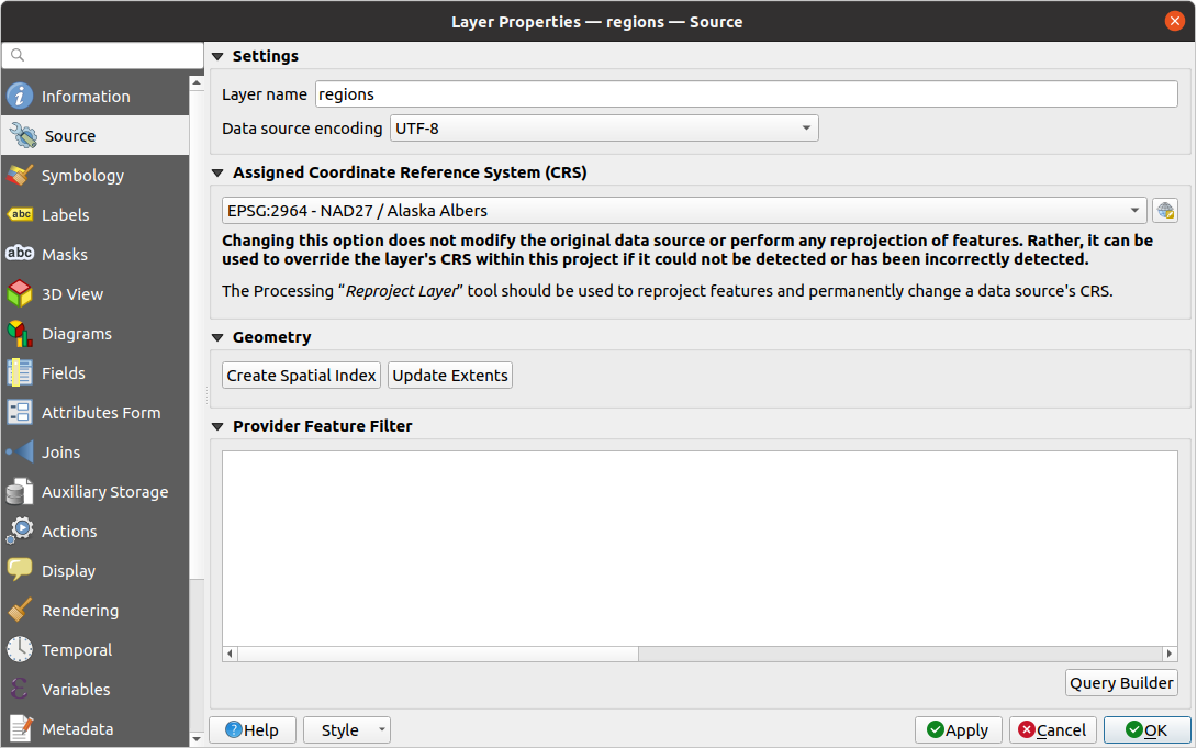
 Select CRS button
(see Seletor do Sistemas de Referência de Coordenadas). Use this process only if the CRS applied to the
layer is a wrong one or if none was applied.
If you wish to reproject your data into another CRS, rather use layer reprojection
algorithms from Processing or Save it into another layer.
Select CRS button
(see Seletor do Sistemas de Referência de Coordenadas). Use this process only if the CRS applied to the
layer is a wrong one or if none was applied.
If you wish to reproject your data into another CRS, rather use layer reprojection
algorithms from Processing or Save it into another layer.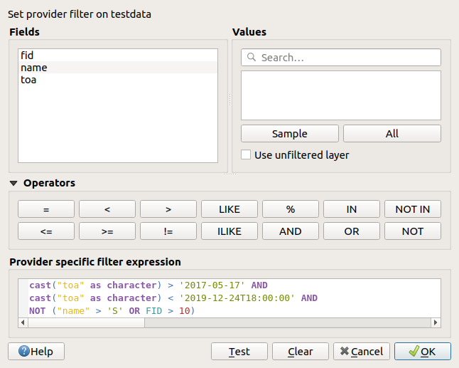
 Filter icon next to it indicating the query used when the mouse hovers over the button.
Double-click the icon opens the Query Builder dialog for edit.
This can also be achieved through the menu.
Filter icon next to it indicating the query used when the mouse hovers over the button.
Double-click the icon opens the Query Builder dialog for edit.
This can also be achieved through the menu. Symbology tab provides you with a comprehensive tool for
rendering and symbolizing your vector data. You can use tools that are
common to all vector data, as well as special symbolizing tools that were
designed for the different kinds of vector data. However all types share the
following dialog structure: in the upper part, you have a widget that helps
you prepare the classification and the symbol to use for features and at
the bottom the Renderização da camada widget.
Symbology tab provides you with a comprehensive tool for
rendering and symbolizing your vector data. You can use tools that are
common to all vector data, as well as special symbolizing tools that were
designed for the different kinds of vector data. However all types share the
following dialog structure: in the upper part, you have a widget that helps
you prepare the classification and the symbol to use for features and at
the bottom the Renderização da camada widget.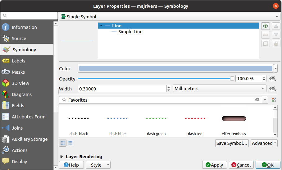
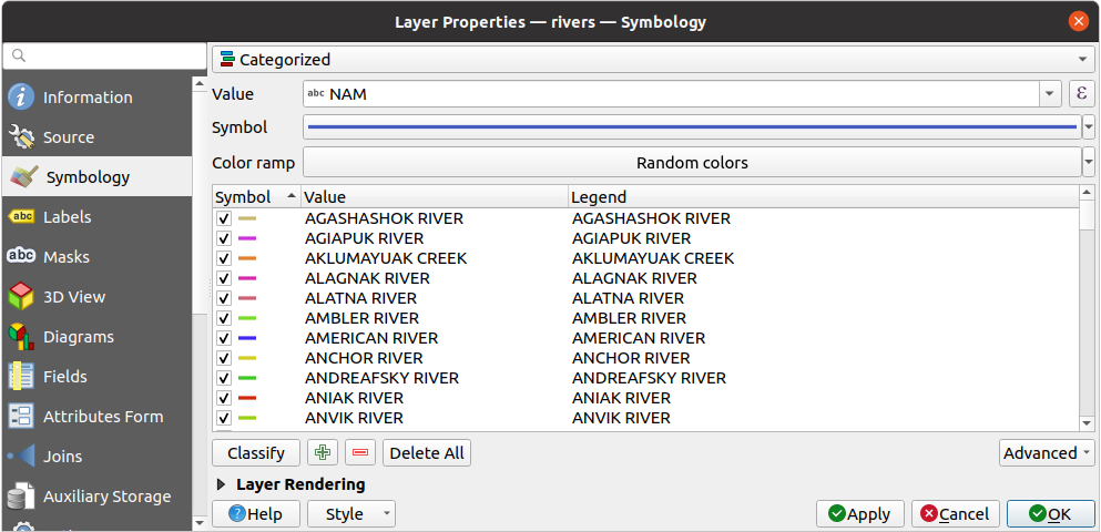
 button.
Using expressions for categorizing avoids the need to create a field for symbology purposes only
(eg, if your classification criteria are derived from one or more attributes).
button.
Using expressions for categorizing avoids the need to create a field for symbology purposes only
(eg, if your classification criteria are derived from one or more attributes). Add new categories,
  Remove
selected categories, Delete All of them or Delete Unused categories.
Remove
selected categories, Delete All of them or Delete Unused categories.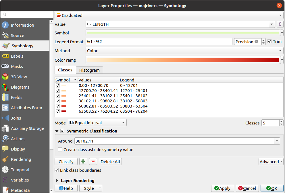
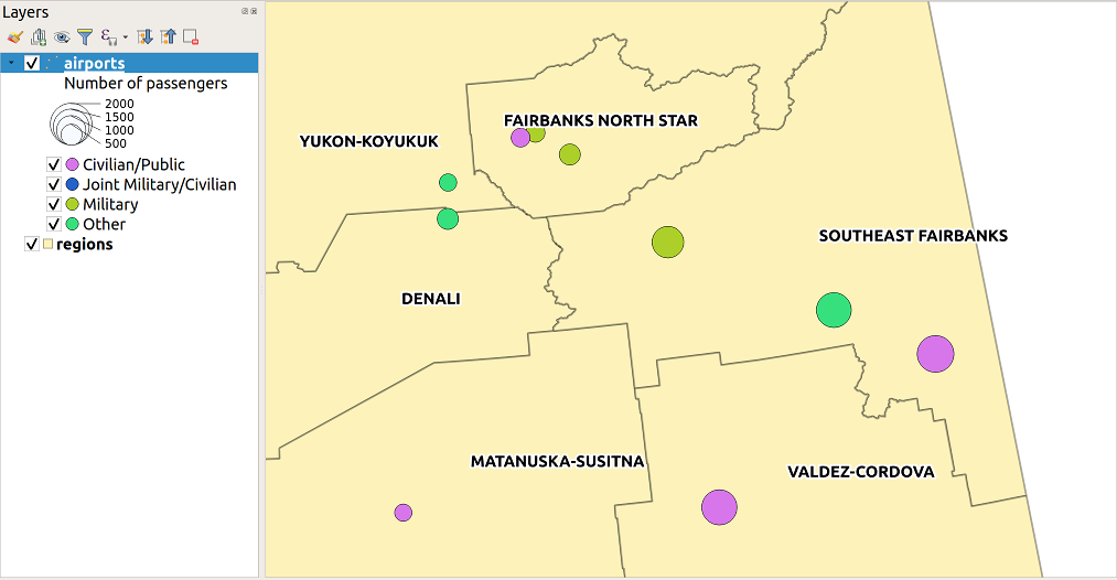
 Rule-based renderer is thus designed
to render all the features from a layer, using symbols whose aspect
reflects the assignment of a selected feature to a fine-grained class.
Rule-based renderer is thus designed
to render all the features from a layer, using symbols whose aspect
reflects the assignment of a selected feature to a fine-grained class. Edit rule or
  Symbols
in the Edit rule dialog to avoid rendering a particular symbol
in the stack.
Symbols
in the Edit rule dialog to avoid rendering a particular symbol
in the stack.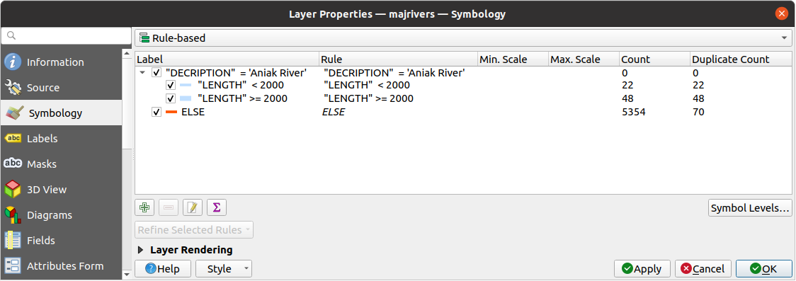
 Point Displacement renderer takes
the point features falling in a given distance tolerance from each other and
places their symbols around their barycenter, following different placement
methods. This can be a convenient way to visualize all the features of a point
layer, even if they have the same location (e.g. amenities in a building).
Point Displacement renderer takes
the point features falling in a given distance tolerance from each other and
places their symbols around their barycenter, following different placement
methods. This can be a convenient way to visualize all the features of a point
layer, even if they have the same location (e.g. amenities in a building).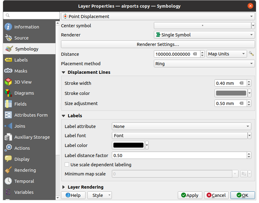
 Point Cluster renderer groups nearby points into a single
rendered marker symbol. Points that fall within a specified distance
from each others are merged into a single symbol.
Points aggregation is made based on the closest group being formed, rather
than just assigning them the first group within the search distance.
Point Cluster renderer groups nearby points into a single
rendered marker symbol. Points that fall within a specified distance
from each others are merged into a single symbol.
Points aggregation is made based on the closest group being formed, rather
than just assigning them the first group within the search distance.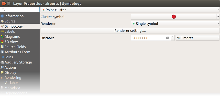
 Merged Features renderer allows area and line
features to be “dissolved” into a single object prior to rendering to ensure that
complex symbols or overlapping features are represented by a uniform and
contiguous cartographic symbol.
Merged Features renderer allows area and line
features to be “dissolved” into a single object prior to rendering to ensure that
complex symbols or overlapping features are represented by a uniform and
contiguous cartographic symbol.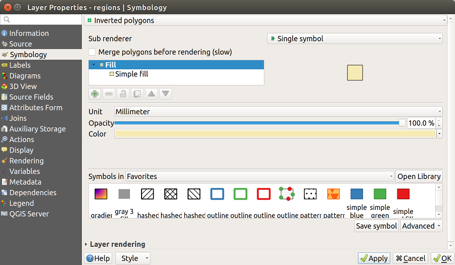
 Heatmap renderer you can create live
dynamic heatmaps for (multi)point layers.
You can specify the heatmap Radius in millimeters, points, pixels, map units or
inches, choose and edit a Color ramp for the heatmap style and use a slider for
selecting a trade-off between render speed and quality. You can also define a
Maximum value limit and Weight points by using a field or an expression.
Heatmap renderer you can create live
dynamic heatmaps for (multi)point layers.
You can specify the heatmap Radius in millimeters, points, pixels, map units or
inches, choose and edit a Color ramp for the heatmap style and use a slider for
selecting a trade-off between render speed and quality. You can also define a
Maximum value limit and Weight points by using a field or an expression. Data defined override to dynamically control Radius and
Maximum value based on the attributes of your data.
For example, the radius of a heatmap point could be determined by its population attribute,
or the maximum value could be based on a temporal range.
Data defined override to dynamically control Radius and
Maximum value based on the attributes of your data.
For example, the radius of a heatmap point could be determined by its population attribute,
or the maximum value could be based on a temporal range.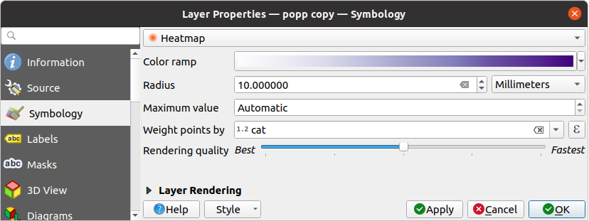
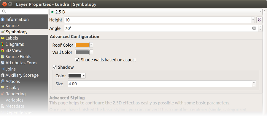
 : You can make the underlying layer in
the map canvas visible with this tool. Use the slider to adapt the visibility
of your vector layer to your needs. You can also make a precise definition of
the percentage of visibility in the menu beside the slider.
: You can make the underlying layer in
the map canvas visible with this tool. Use the slider to adapt the visibility
of your vector layer to your needs. You can also make a precise definition of
the percentage of visibility in the menu beside the slider.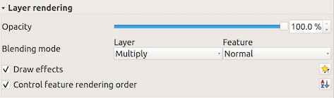
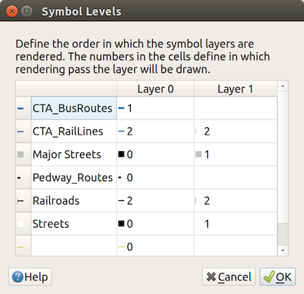
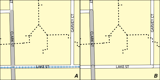
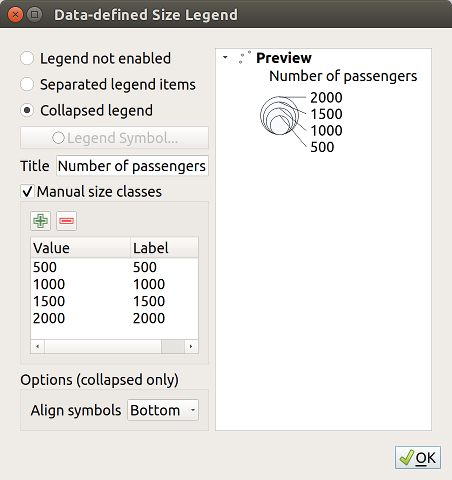
 Is Animated to enable animation for the symbol

 Customize effects button. That will open
the Effect Properties Dialog (see Fig. 12.19). The following
effect types, with custom options are available:
Customize effects button. That will open
the Effect Properties Dialog (see Fig. 12.19). The following
effect types, with custom options are available: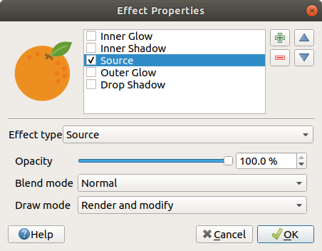
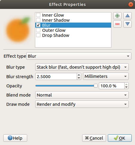
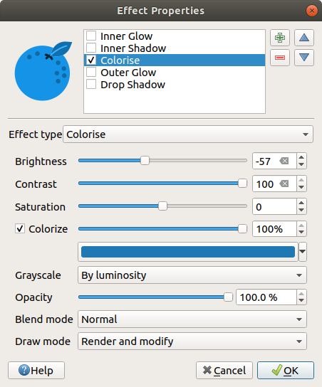
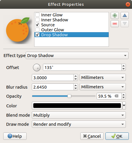
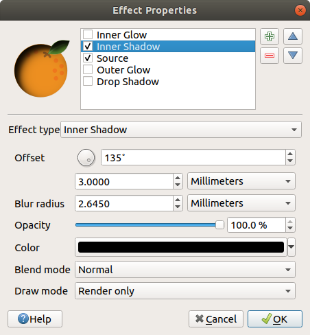
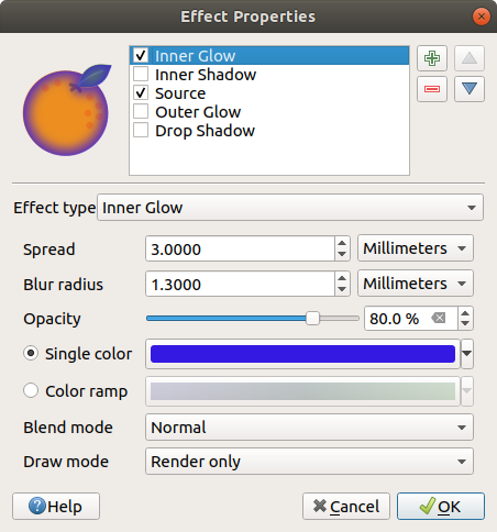
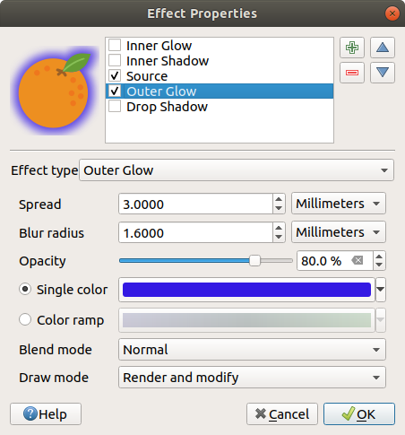
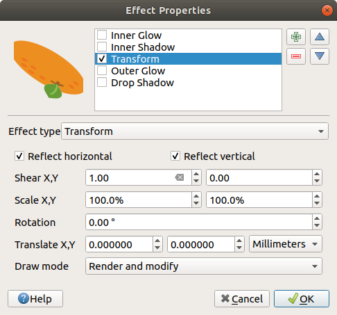
 Configure project labeling rules button:
helps you control interactions between labels and features across the layers in the project.
More details at Configuring project labeling rules.
Configure project labeling rules button:
helps you control interactions between labels and features across the layers in the project.
More details at Configuring project labeling rules. Automated placement settings (applies to all layers) button:
configure general properties on label placement and conflicts resolution.
More details at Configurando o mecanismo de posicionamento automatizado.
Automated placement settings (applies to all layers) button:
configure general properties on label placement and conflicts resolution.
More details at Configurando o mecanismo de posicionamento automatizado. No labels: the default value, showing no labels
from the layer
No labels: the default value, showing no labels
from the layer Single labels: Show labels on the map using a single
attribute or an expression
Single labels: Show labels on the map using a single
attribute or an expression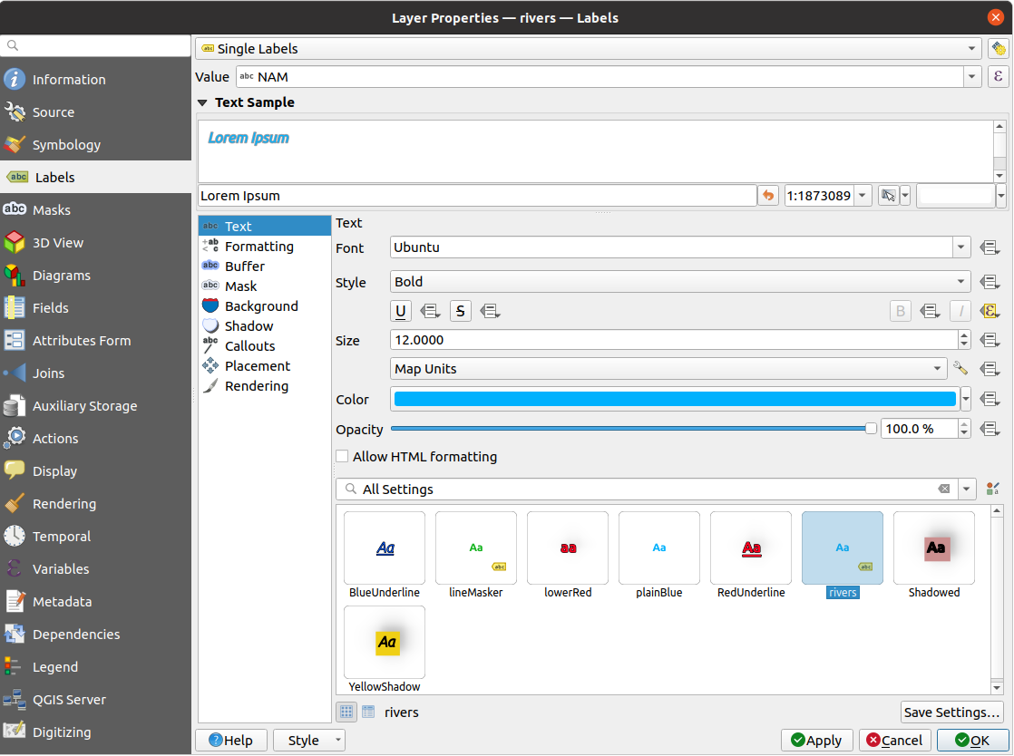


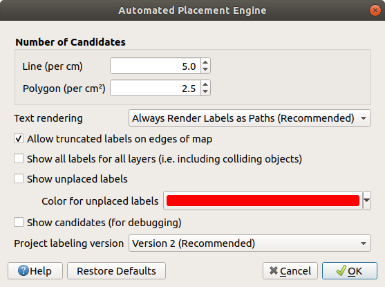
 Rule-based labeling option in the main
drop-down list from the Labels tab
Rule-based labeling option in the main
drop-down list from the Labels tab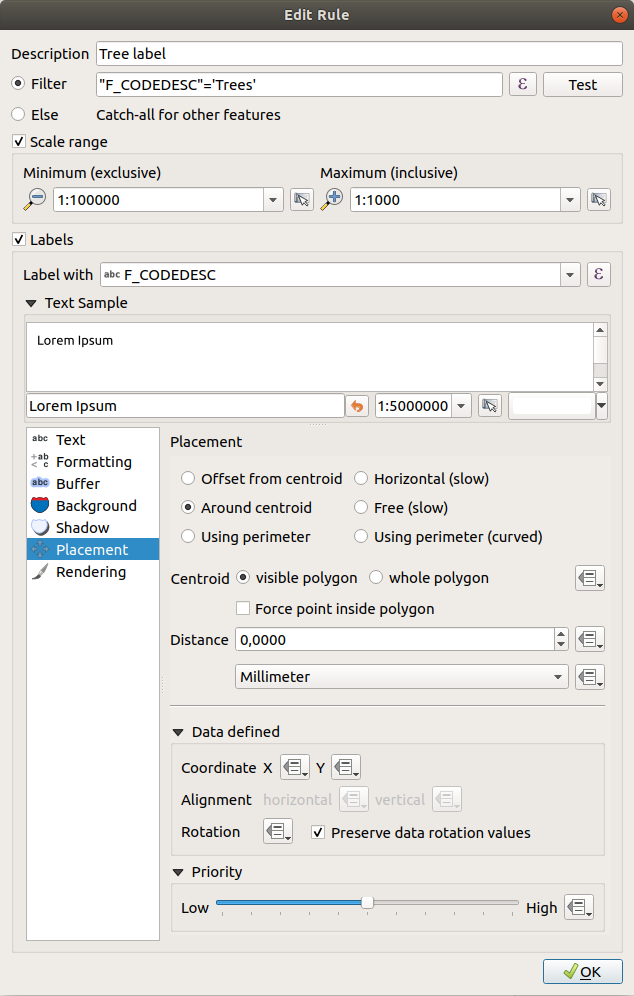
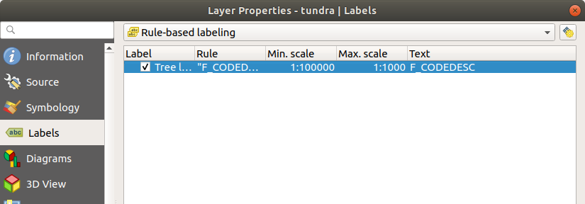
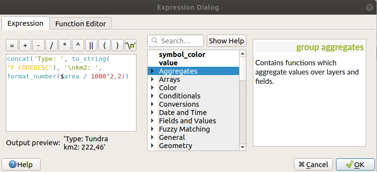
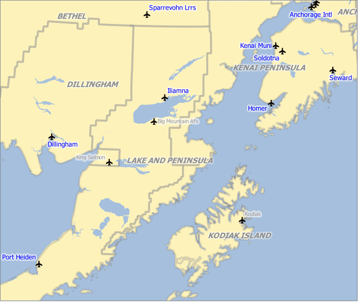
 diagram properties:
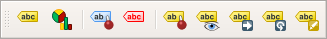
 Highlight Pinned Labels, Diagrams and Callouts.
If the vector layer of the item is editable, then the highlighting is green,
otherwise it’s blue.
Highlight Pinned Labels, Diagrams and Callouts.
If the vector layer of the item is editable, then the highlighting is green,
otherwise it’s blue. Toggle Display of Unplaced Labels: Allows to
determine whether any important labels are missing from the maps (e.g. due
to overlaps or other constraints). They are displayed with a customizable
color (see Configurando o mecanismo de posicionamento automatizado).
Toggle Display of Unplaced Labels: Allows to
determine whether any important labels are missing from the maps (e.g. due
to overlaps or other constraints). They are displayed with a customizable
color (see Configurando o mecanismo de posicionamento automatizado). Pin/Unpin Labels and Diagrams. By clicking or dragging an
area, you pin overlaid items. If you click or drag an area holding Shift,
the items are unpinned. Finally, you can also click or drag an area holding
Ctrl to toggle their pin status.
Pin/Unpin Labels and Diagrams. By clicking or dragging an
area, you pin overlaid items. If you click or drag an area holding Shift,
the items are unpinned. Finally, you can also click or drag an area holding
Ctrl to toggle their pin status. Show/Hide Labels and Diagrams. If you click on the items,
or click and drag an area holding Shift, they are hidden.
When an item is hidden, you just have to click on the feature to restore its
visibility. If you drag an area, all the items in the area will be restored.
Show/Hide Labels and Diagrams. If you click on the items,
or click and drag an area holding Shift, they are hidden.
When an item is hidden, you just have to click on the feature to restore its
visibility. If you drag an area, all the items in the area will be restored. Move a Label, Diagram or Callout: click to select
the item and click to move it to the desired place. The new coordinates are
stored in auxiliary fields.
Selecting the item with this tool and hitting the Delete key
will delete the stored position value.
Move a Label, Diagram or Callout: click to select
the item and click to move it to the desired place. The new coordinates are
stored in auxiliary fields.
Selecting the item with this tool and hitting the Delete key
will delete the stored position value. Rotate a Label. Click to select the label and click again
to apply the desired rotation. Likewise, the new angle is stored in an auxiliary
field. Selecting a label with this tool and hitting the
Delete key will delete the rotation value of this label.
Rotate a Label. Click to select the label and click again
to apply the desired rotation. Likewise, the new angle is stored in an auxiliary
field. Selecting a label with this tool and hitting the
Delete key will delete the rotation value of this label. Change Label Properties. It opens a dialog to change the
clicked label properties; it can be the label itself, its coordinates, angle,
font, size, multiline alignment … as long as this property has been mapped
to a field. Here you can set the option to
Change Label Properties. It opens a dialog to change the
clicked label properties; it can be the label itself, its coordinates, angle,
font, size, multiline alignment … as long as this property has been mapped
to a field. Here you can set the option to 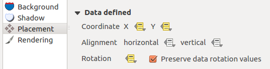
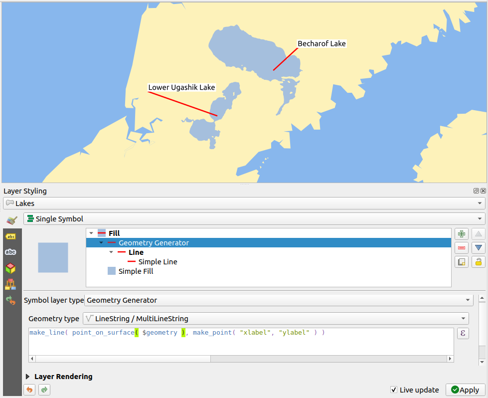
 No diagrams: the default value with no diagram
displayed over the features;
No diagrams: the default value with no diagram
displayed over the features; Pie chart, a circular statistical graphic divided into
slices to illustrate numerical proportion. The arc length of each slice is
proportional to the quantity it represents;
Pie chart, a circular statistical graphic divided into
slices to illustrate numerical proportion. The arc length of each slice is
proportional to the quantity it represents; Text diagram, a horizontally divided circle showing statistic
values inside;
Text diagram, a horizontally divided circle showing statistic
values inside; Histogram, bars of varying colors for each attribute
aligned next to each other;
Histogram, bars of varying colors for each attribute
aligned next to each other; Stacked bars, stacks bars of varying colors for each
attribute on top of each other vertically or horizontally;
Stacked bars, stacks bars of varying colors for each
attribute on top of each other vertically or horizontally; Stacked diagram, stacks diagrams of equal or varying
types, next to each other, vertically or horizontally. More details at
Stacked Diagrams.
Stacked diagram, stacks diagrams of equal or varying
types, next to each other, vertically or horizontally. More details at
Stacked Diagrams.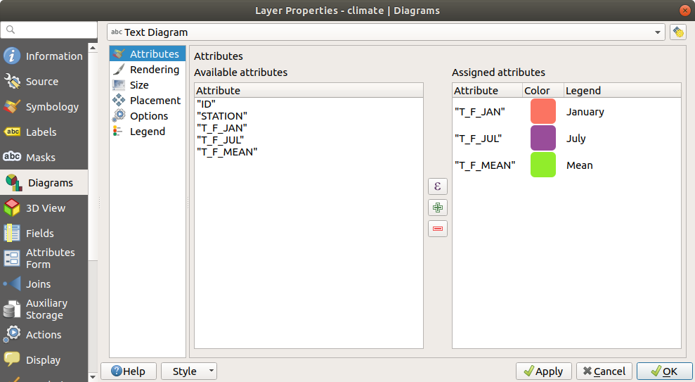
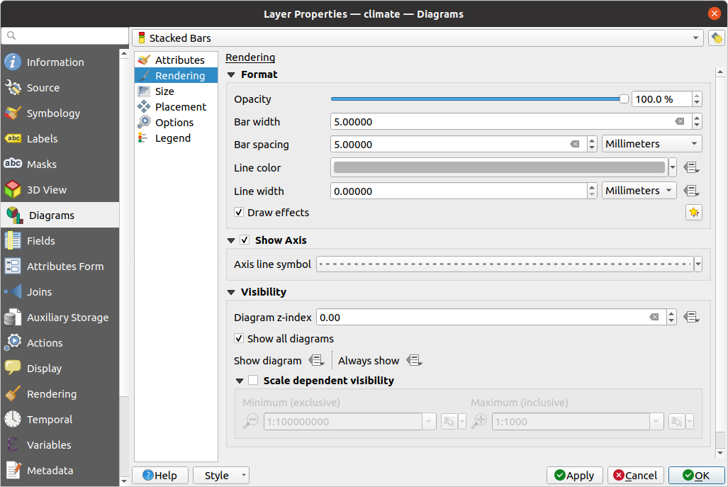
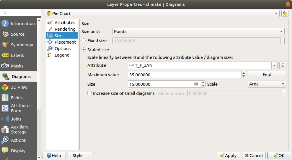
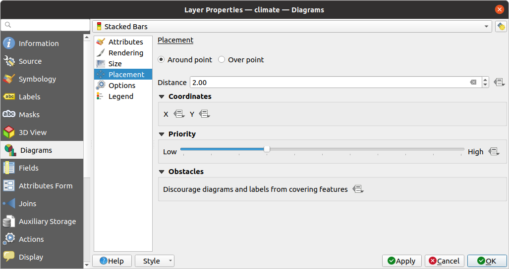

 Masks tab helps you configure the current layer
symbols overlay with other symbol layers or labels, from any layer.
This is meant to improve the readability of symbols and labels whose colors
are close and can be hard to decipher when overlapping; it adds a custom and
transparent mask around the items to “hide” parts of the symbol layers of
the current layer.
Masks tab helps you configure the current layer
symbols overlay with other symbol layers or labels, from any layer.
This is meant to improve the readability of symbols and labels whose colors
are close and can be hard to decipher when overlapping; it adds a custom and
transparent mask around the items to “hide” parts of the symbol layers of
the current layer.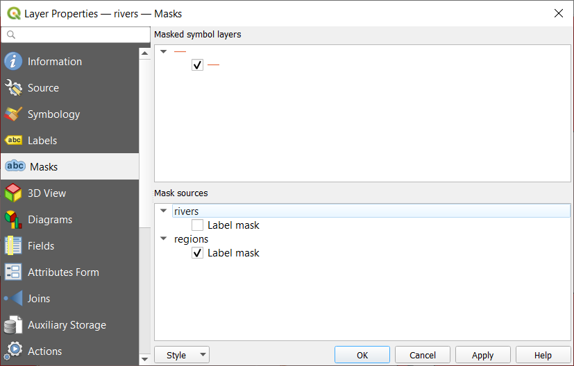
 3D View tab provides settings for vector layers that should
be depicted in the 3D Map view tool.
3D View tab provides settings for vector layers that should
be depicted in the 3D Map view tool.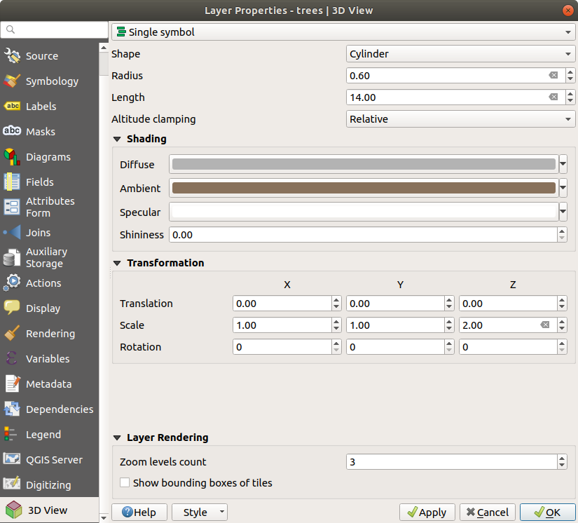
 Fields tab provides information on
fields related to the layer and helps you organize them.
Fields tab provides information on
fields related to the layer and helps you organize them. New field, the Comment option is
available only for data sources that allow editing comments
(See Entradas no banco de dados for more details).
You can also set aliases within Add Field dialog, for supported
OGR formats (GeoPackage and ESRI File Geodatabase).
New field, the Comment option is
available only for data sources that allow editing comments
(See Entradas no banco de dados for more details).
You can also set aliases within Add Field dialog, for supported
OGR formats (GeoPackage and ESRI File Geodatabase).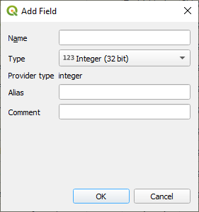
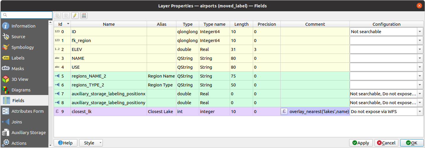
 Attributes Form tab helps you set up the form to
display when creating new features, editing or querying existing one.
This affects them in both table and form views.
You can define:
Attributes Form tab helps you set up the form to
display when creating new features, editing or querying existing one.
This affects them in both table and form views.
You can define: Show field aliases instead of names button allows
you to toggle field aliases and field names.
Show field aliases instead of names button allows
you to toggle field aliases and field names.
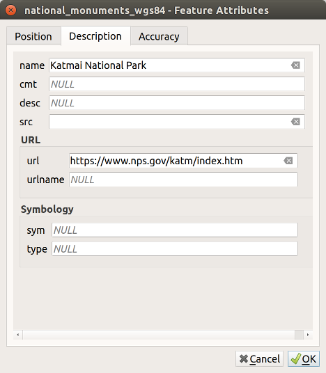
 Invert selection button.
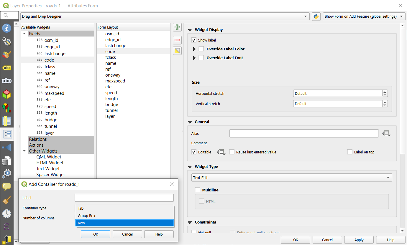

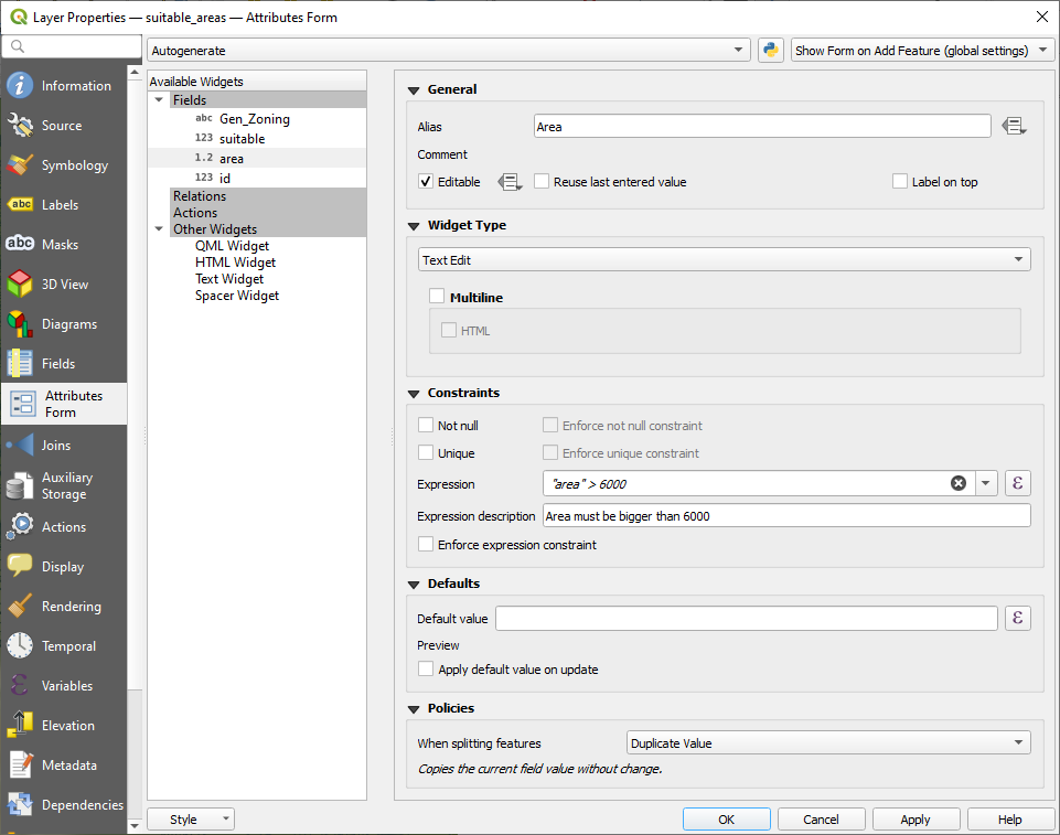
 Joins tab allows you to associate features
of the current layer to features from another loaded vector layer (or table).
The join is based on an attribute that is shared by the layers,
in a one-to-one relationship.
For more details on joins, please read Joining features between two layers.
Joins tab allows you to associate features
of the current layer to features from another loaded vector layer (or table).
The join is based on an attribute that is shared by the layers,
in a one-to-one relationship.
For more details on joins, please read Joining features between two layers.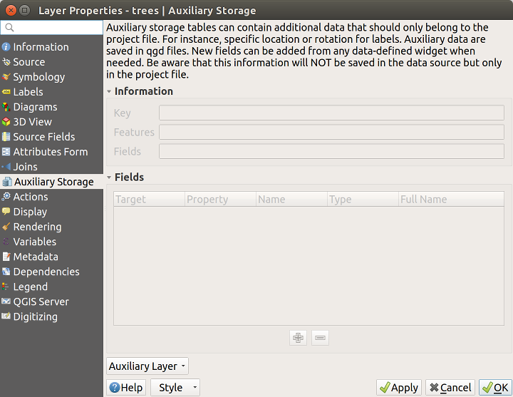
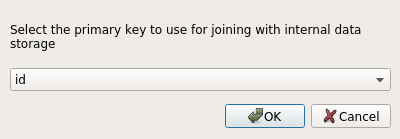
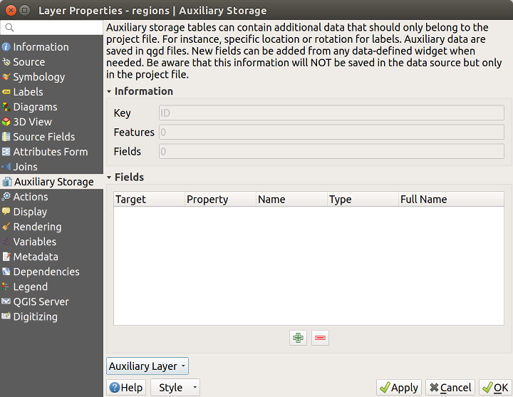
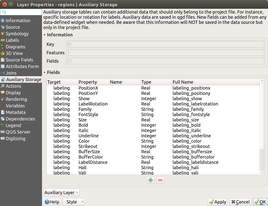
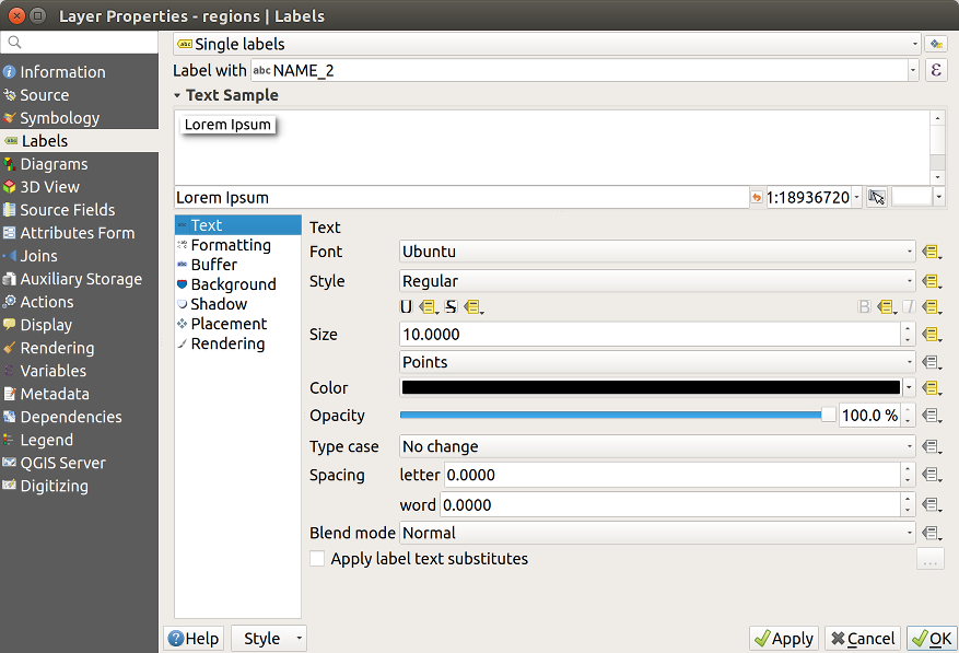
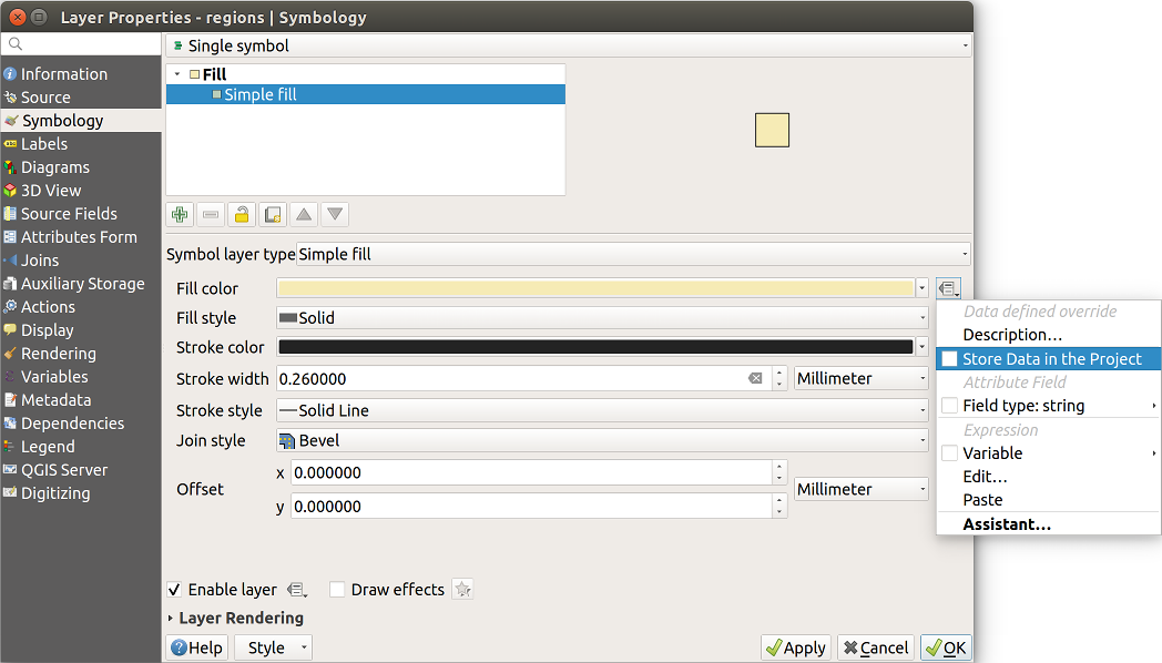
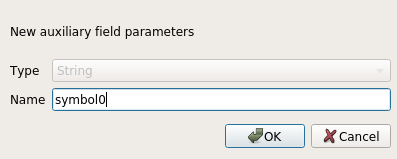
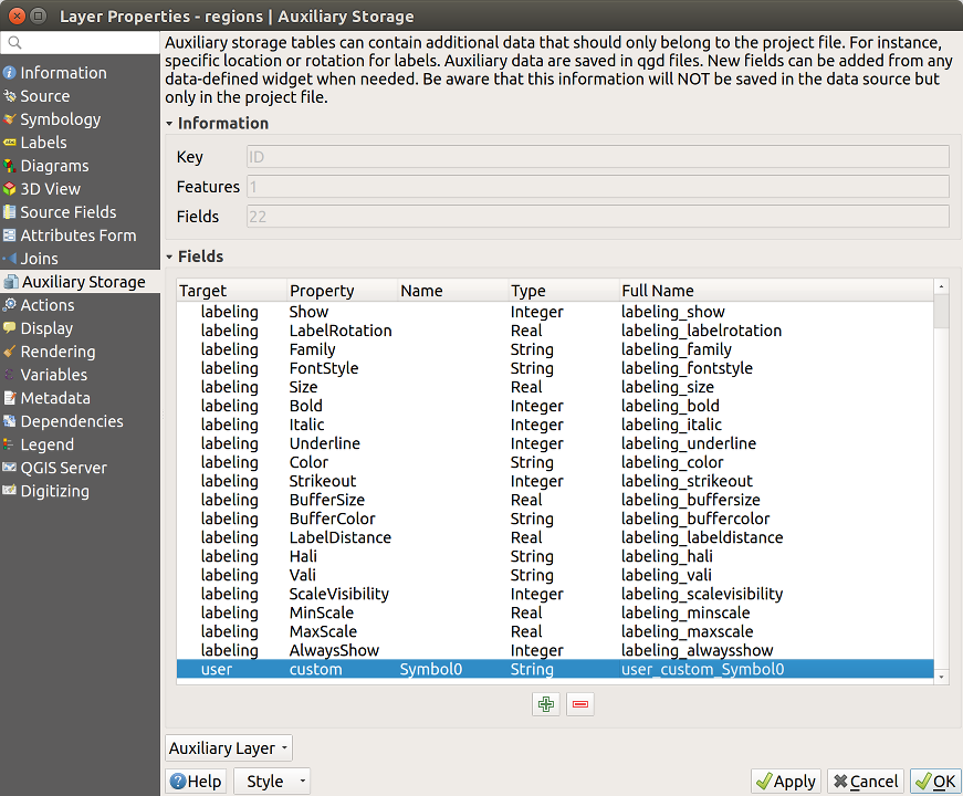
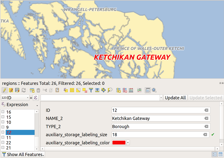
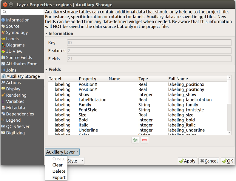
 Actions tab provides the ability to perform an action
based on the attributes of a feature.
This can be used to perform any number of actions, for example,
running a program with arguments built from the attributes of a feature
or passing parameters to a web reporting tool.
Actions tab provides the ability to perform an action
based on the attributes of a feature.
This can be used to perform any number of actions, for example,
running a program with arguments built from the attributes of a feature
or passing parameters to a web reporting tool.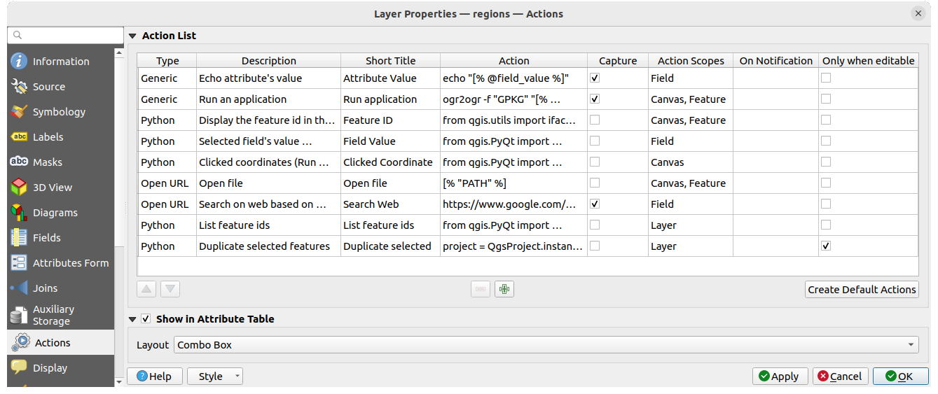
 Duplicate an action
to open the Duplicate Action dialog. You must have selected at least one existing action
in order to create a duplicate.
Duplicate an action
to open the Duplicate Action dialog. You must have selected at least one existing action
in order to create a duplicate. Identify Features tool
(see Identificando Feições for more information);
Identify Features tool
(see Identificando Feições for more information); or perhaps
  ). The layer in question has fields for a species name
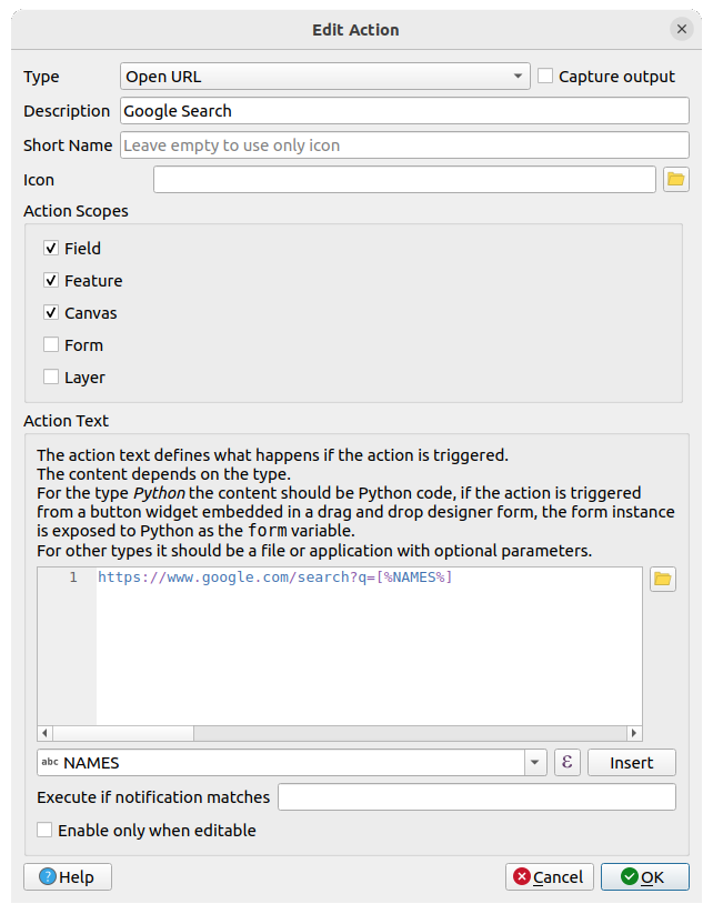
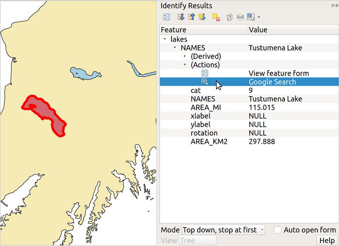
 Display tab helps you configure fields to use for
feature identification:
Display tab helps you configure fields to use for
feature identification: Show Map Tips icon pressed.
Applicable when
Show Map Tips icon pressed.
Applicable when 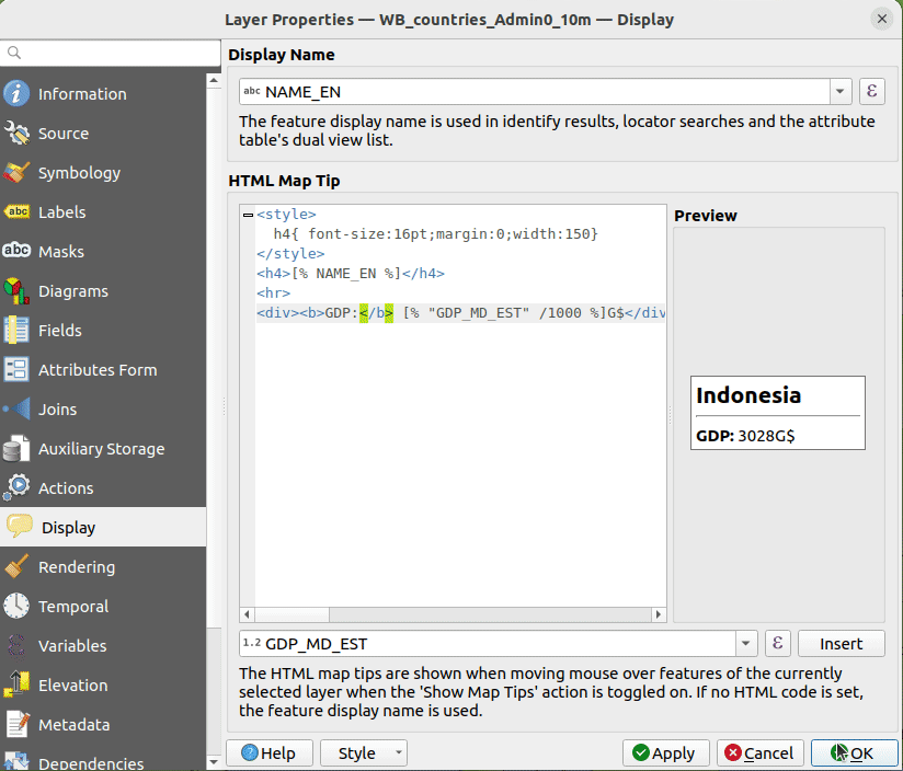
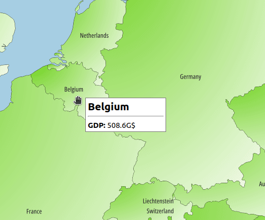
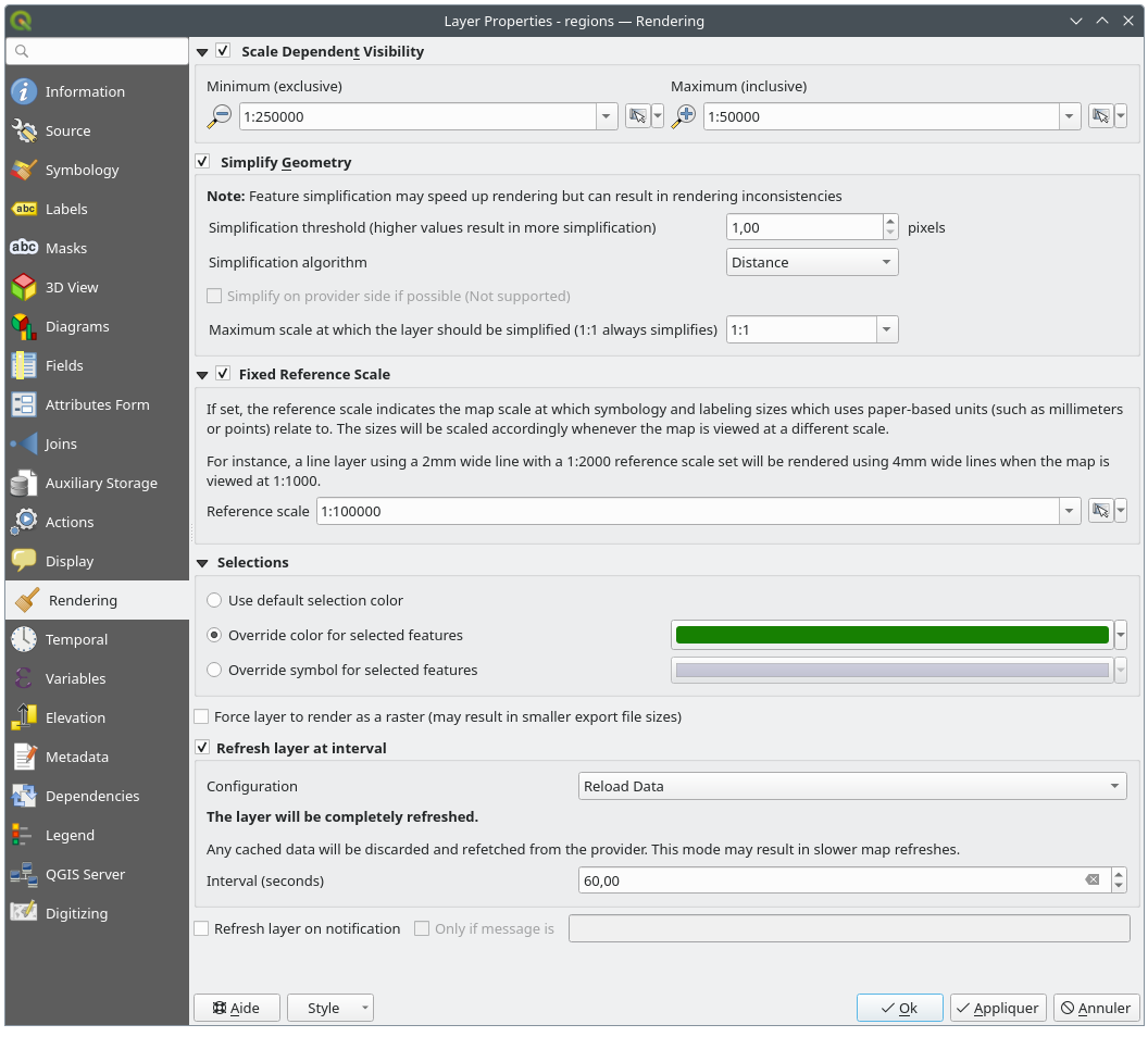
 Rendering tab offers following properties:
 Set to current canvas scale button helps you
use the current map canvas scale as boundary of the range visibility.
See Visibility Scale Selector for more information.
Set to current canvas scale button helps you
use the current map canvas scale as boundary of the range visibility.
See Visibility Scale Selector for more information. Temporal tab provides options to control
the rendering of the layer over time. Such dynamic rendering requires the
temporal navigation to be enabled over the map canvas.
Temporal tab provides options to control
the rendering of the layer over time. Such dynamic rendering requires the
temporal navigation to be enabled over the map canvas.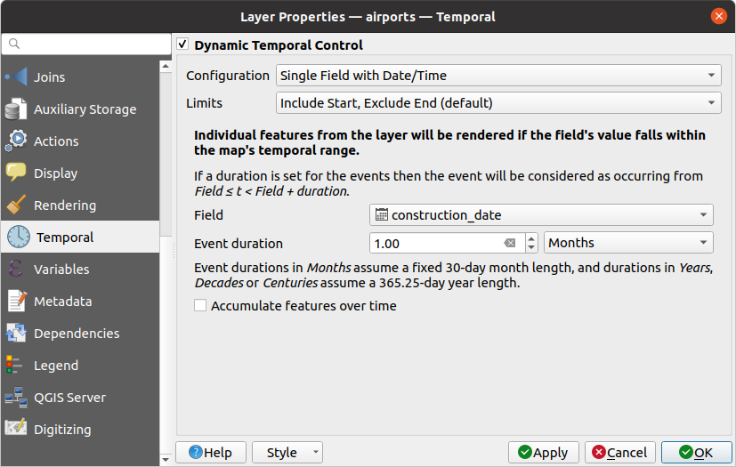
 Elevation tab provides options to control
the layer elevation properties within a 3D map view
and its appearance in the profile tool charts.
Specifically, you can set:
Elevation tab provides options to control
the layer elevation properties within a 3D map view
and its appearance in the profile tool charts.
Specifically, you can set: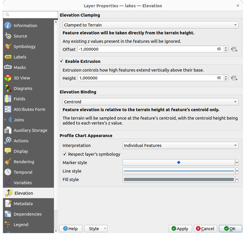
 Metadata tab provides you with options
to create and edit a metadata report on your layer.
See Metadados for more information.
Metadata tab provides you with options
to create and edit a metadata report on your layer.
See Metadados for more information. Dependencies tab allows to declare data
dependencies between layers. A data dependency occurs when a data modification
in a layer, not by direct user manipulation, may modify data of other layers.
This is the case for instance when geometry of a layer is updated by a
database trigger or custom PyQGIS scripting after modification of another
layer’s geometry.
Dependencies tab allows to declare data
dependencies between layers. A data dependency occurs when a data modification
in a layer, not by direct user manipulation, may modify data of other layers.
This is the case for instance when geometry of a layer is updated by a
database trigger or custom PyQGIS scripting after modification of another
layer’s geometry. Legend properties tab provides you with advanced
settings for the Layers panel and/or the print
layout legend. These options include:
Legend properties tab provides you with advanced
settings for the Layers panel and/or the print
layout legend. These options include: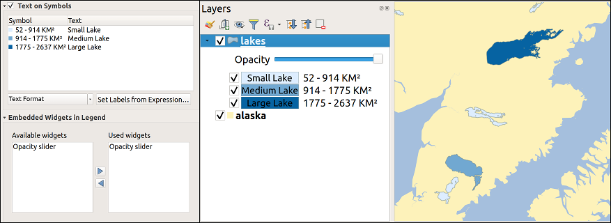
 QGIS Server tab consists of Description,
Attribution, Metadata URL, and Legend URL
sections.
QGIS Server tab consists of Description,
Attribution, Metadata URL, and Legend URL
sections.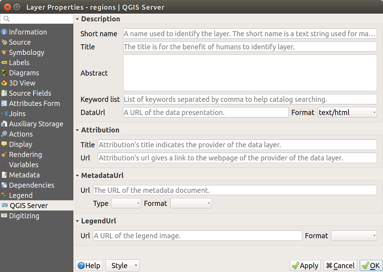
 Digitizing tab gives access to options that help
to ensure the quality of digitized geometries.
Digitizing tab gives access to options that help
to ensure the quality of digitized geometries.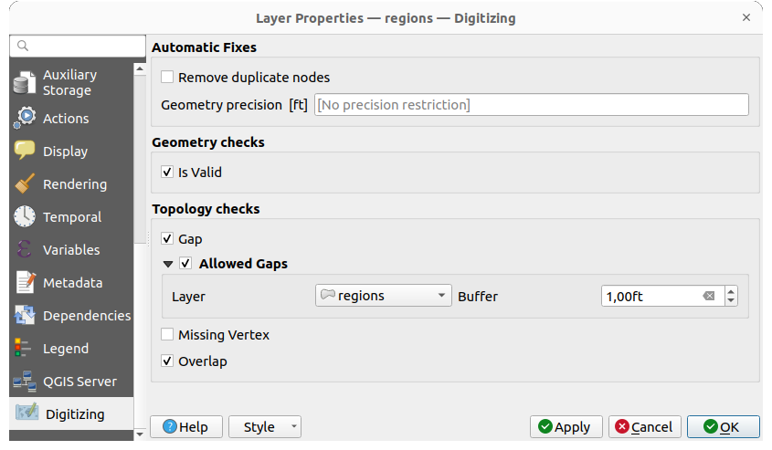
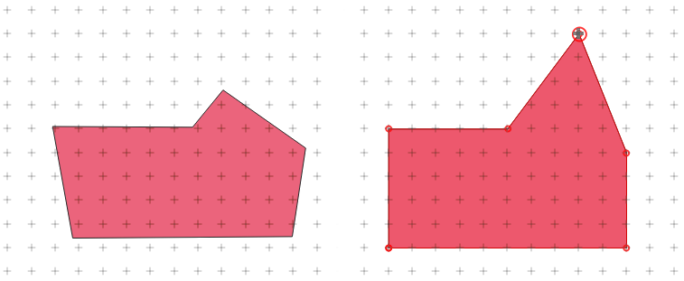

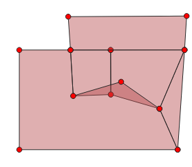
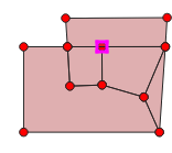
 Zoom to Feature(s)
 Zoom to problem