Important

La traduction est le fruit d’un effort communautaire auquel vous pouvez vous joindre. Cette page est actuellement traduite à 28.57%.

14.4. Leçon : Mettre à jour les massifs forestiers

Now that you have digitized the information from the old inventory maps and added the corresponding information to the forest stands, the next step is to create the inventory of the current state of the forest.

You will digitize new forest stands using an aerial photo. As with the previous lesson, you will use an aerial Color Infrared (CIR) photograph. This type of imagery, where the infrared light is recorded instead of the blue light, is widely used to study vegetated areas.

Après la numérisation des massifs de forêt, vous ajouterez des informations telles que les nouvelles contraintes données par les réglementations de conservation.

The goal for this lesson: To digitize a new set of forest stands from CIR aerial photographs and add information from other datasets.

14.4.1. ★☆☆ Comparing the Old Forest Stands to Current Aerial Photographs

The National Land Survey of Finland has an open data policy that allows you downloading a variety of geographical data like aerial imagery, traditional topographic maps, DEM, LiDAR data, etc. The service can be accessed in English here. The aerial image used in this exercise has been created from two orthorectified CIR images downloaded from that service (M4134F_21062012 and M4143E_21062012).

1. Open QGIS and set the project’s CRS to ETRS89 / ETRS-TM35FIN in Project ► Properties… ► CRS

2. Add the CIR image rautjarvi_aerial.tif to the project:

   1. Go to the exercise_data\forestry\ folder using your file manager browser

   2. Drag and drop the file rautjarvi_aerial.tif onto your project

3. Save the QGIS project as digitizing_2012.qgs

Les images CIR sont de 2012. Vous pouvez comparer les massifs qui ont été créés en 1994 avec la situation d’il y a environ 20 ans.

1. Add the forest_stands_1994.shp layer created in the previous lesson:

   1. Go to the exercise_data\forestry\ folder using your file manager browser

   2. Drag and drop the file forest_stands_1994.shp onto your project

2. Set the symbology for the layer so that you can see through your polygons:

   1. Right click forest_stands_1994

   2. Select Properties

   3. Go to the Symbology tab

   4. Set Fill color to transparent fill

   5. Set Stroke color to purple

   6. Set Stroke width to 0.50 mm

3. Étudiez comment les anciens massifs de forêt suivent (ou non) ce que vous pouvez visuellement interpréter comme de la forêt homogène.

4. Zoomez et bouger autour de la zone. Vous remarquerez probablement que certains des anciens massifs de forêt pourraient correspondre à l’image alors que d’autres non.

   This is a normal situation, as some 20 years have passed and different forest operations have been carried out (harvesting, thinning…). It is also possible that the forest stands looked homogeneous back in 1992 to the person who digitized them but as time has passed some forest has developed in different ways. It is also possible that that forest inventory priorities back then were different from those of today.

Ensuite, vous créerez de nouveaux massifs de forêt pour cette image sans utiliser les anciens. Plus tard, vous pourrez les comparer pour voir les différences.

14.4.2. ★☆☆ Interpreting the CIR Image

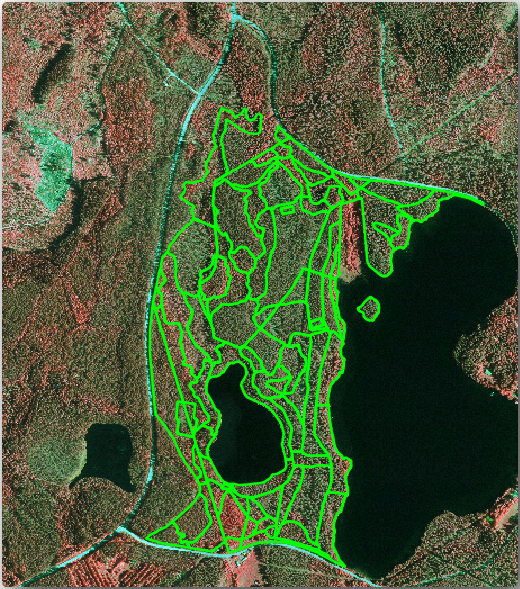
Numérisons la même zone qui était couverte par l’ancien inventaire, limitée par les routes et par le lac. Vous n’avez pas besoin de numériser l’entier de la zone, comme dans l’exercice précédent, vous pouvez commencer avec un fichier vectoriel qui contient déjà la plupart des massifs de forêt.

1. Remove the layer forest_stands_1994

2. Add the file exercise_data\forestry\forest_stands_2012.shp to the project

3. Set the styling of this layer so that the polygons have no fill and the borders are visible

   1. Open Properties dialog of the forest_stands_2012 layer

   2. Go to the Symbology tab

   3. Set Fill color to transparent fill

   4. Set Stroke color to green

   5. Set Stroke width to 0.50 mm

   

   
   

You can see that the northern section of the inventory area is still missing. Your task is to digitize the missing forest stands.

Before you start, spend some time reviewing the forest stands already digitized and the corresponding forest in the image. Try to get an idea about how the stands borders are decided, it helps if you have some forestry knowledge.

Some points to consider:

• Which forests have deciduous species (in Finland these are mostly birch forests) and which ones have conifers (in this area these are pine or spruce)? In CIR images, deciduous species usually show up as a bright red color whereas conifers show as a dark green color.

• How old is the forest? The size of the tree crowns can be identified in the imagery.

• How dense are the different forest stands? A forest stand where a thinning operation has recently been done would show spaces between the tree crowns and should be easy to differentiate from other forest stands around it.

• Des zones bleutées indiquent des terrains stériles, routes et zones urbaines, les cultures qui ne sont pas ouvertes à croître, etc.

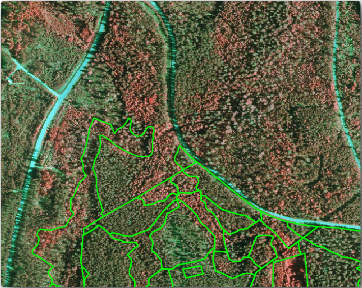
• Don’t use zooms too close to the image when trying to identify forest stands. A scale between 1:3 000 and 1:5 000 should be enough for this imagery. See the image below (1:4000 scale):

14.4.3. ★☆☆ Try Yourself: Digitizing Forest Stands from CIR Imagery

When digitizing the forest stands, you should try to get forest areas that are as homogeneous as possible in terms of tree species, forest age, stand density… Don’t be too detailed though, or you will end up making hundreds of small forest stands - and that would not be useful at all. You should try to get stands that are meaningful in the context of forestry, not too small (at least 0.5 ha) but not too big either (no more than 3 ha).

With these points in mind, you can now digitize the missing forest stands.

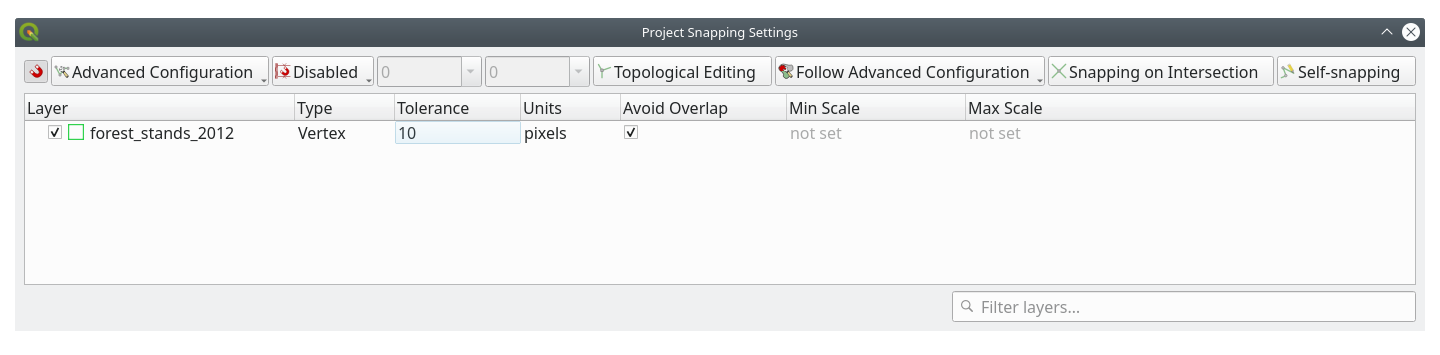
1. Set up the snapping and topology options:

   1. Allez au menu Projet ► Options d’accrochage….

   2. Cochez sur ^{Activer l’accrochage} et sélectionnez Configuration avancée

   3. Check the forest_stands_2012 layer

      1. Set Type to Vertex

      2. Set Tolerance to 10

      3. Set Units to pixels

      4. Check the box under Avoid Overlap

      5. Appuyer sur Édition topologique

      6. Choisissez Suivre la configuration avancée

      7. Fermez la fenêtre

      

2. Select the forest_stands_2012 layer on the Layers list

3. Click the ^{Toggle Editing} button to enable editing

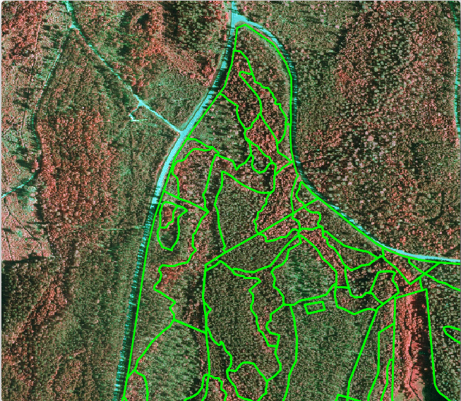
4. Start digitizing using the same techniques as in the previous lesson. The only difference is that you don’t have any point layer that you are snapping to. For this area you should get around 14 new forest stands. While digitizing, fill in the StandID field with numbers starting at 901.

5. Quand vous avez terminé, votre couche devrait ressembler à quelque chose comme ça :

   

Now you have a new set of polygons showing the different forest stands in 2012 - as interpreted from the CIR images. However, you are missing the forest inventory data. For that you will need to visit the forest and get some sample data that you will use to estimate the forest attributes for each of the forest stands. You will see how to do that in the next lesson.

You can add some extra information about conservation regulations that need to be taken into account for this area.

14.4.4. ★☆☆ Follow Along: Updating Forest Stands with Conservation Information

For the area you are working in, there are some conservation regulations that must be taken into account when doing the forest planning:

• Deux emplacements d’une espèce protégée d’écureuil volant de Sibérie (Pteromys volans) ont été identifiés. Selon le règlement, une zone de 15 mètres autours des lieux devrait restée intacte.

• A riparian forest of special interest that is growing along a stream in the area must be protected. In a visit to the field, it was found that 20 meters to both sides of the stream must be protected.

You have a vector file containing the information about the squirrel locations and another containing the digitized stream running from the North area towards the lake.

1. From the exercise_data\forestry\ folder, add the squirrel.shp and stream.shp files to the project.

2. Use the ^{Open Attribute Table} tool to view the squirrel layer

   Vous pouvez voir qu’il y a deux emplacements qui sont définis comme écureuil volant de Sibérie, et que la zone à protéger est indiquée par une distance de 15 mètres des emplacements.

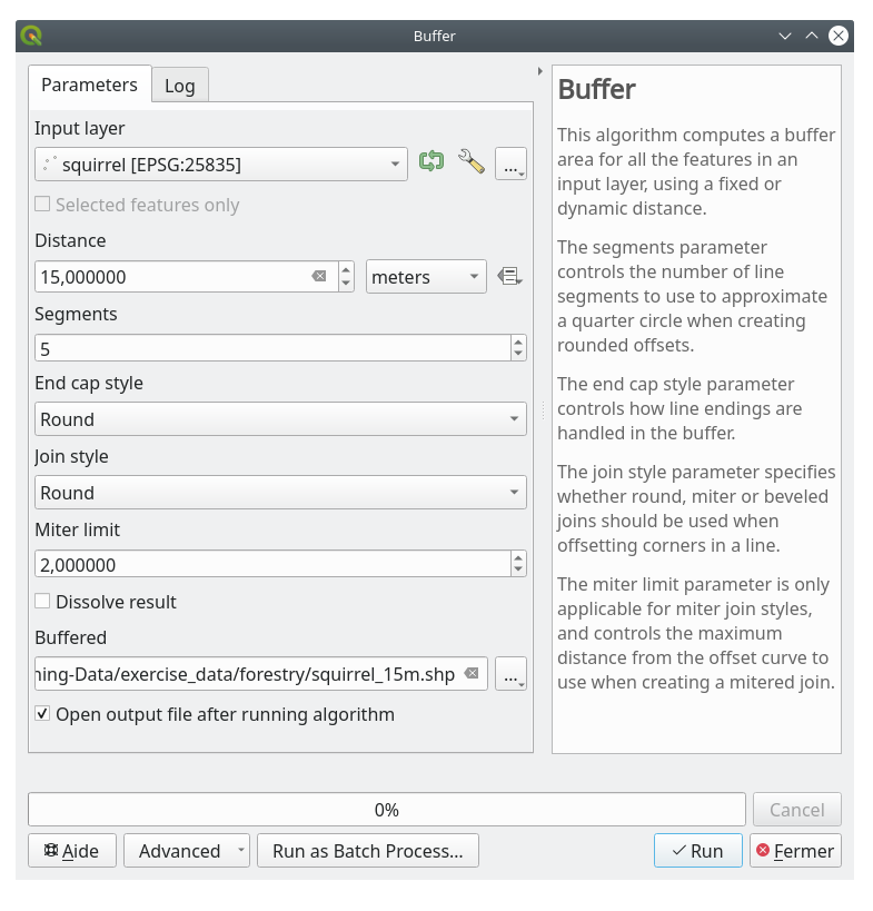
Let’s more accurately delimitate that area to protect. We will create a buffer around the point locations, using the protection distance.

1. Ouvrez Vecteur ► Outils de géotraitement ► Tampon.

2. Set Input layer to squirrel

3. Set Distance to 15 meters

4. Set Buffered to exercise_data\forestry\squirrel_15m.shp

5. Check Open output file afer running algorithm

6. Cliquez sur Exécuter

7. Once the process is completed, click Close

   

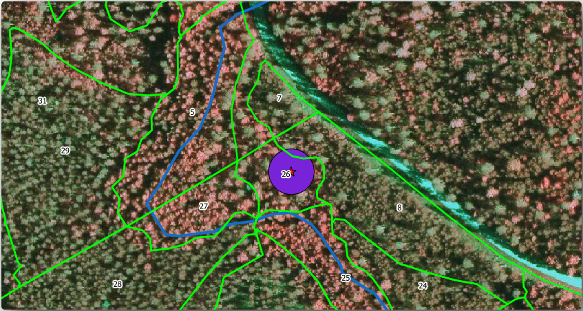
If you zoom in to the location in the northern part of the area, you will notice that the buffer area extends over two neighbouring stands. This means that whenever a forest operation takes place in that stand, the protected location should also be taken into account.

For the protection of the squirrels locations, you are going to add a new attribute (column) to your new forest stands that will contain information about locations that have to be protected. This information will then be available whenever a forest operation is planned, and the field team will be able to mark the area that has to be left untouched before the work starts.

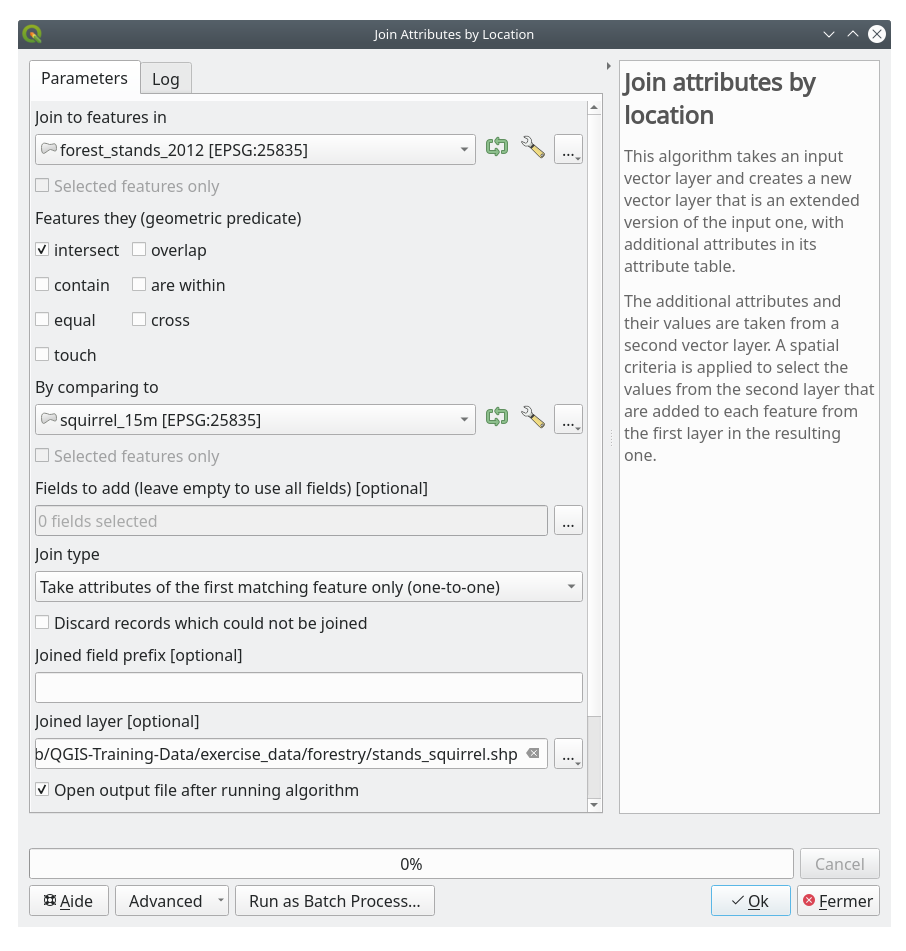
To join the information about the squirrels to your forest stands, you can use the Join attributes by location algorithm:

1. Ouvrez Vecteur ► Outils de gestion de données ► Joindre les attributs par localisation.

2. Set Join to features in to forest_stands_2012

3. In Geometric predicate, check intersect

4. Set By comparing to to squirrel_15m

5. Set Join type as Take attributes of the first matching feature only (one-to-one)

6. Leave unchecked Discard records which could not be joined

7. Set Joined layer to exercise_data\forestry\stands_squirrel.shp

8. Check Open output file afer running algorithm

9. Cliquez sur Exécuter

10. Once the process is completed, you can Close the dialog.

    

Now you have a new forest stands layer, stands_squirrel.shp showing the protection information for the Siberian flying squirrel.

1. Open the attribute table of the stands_squirrel layer

2. Sort the table by clicking on point_pr field in the table header.

   

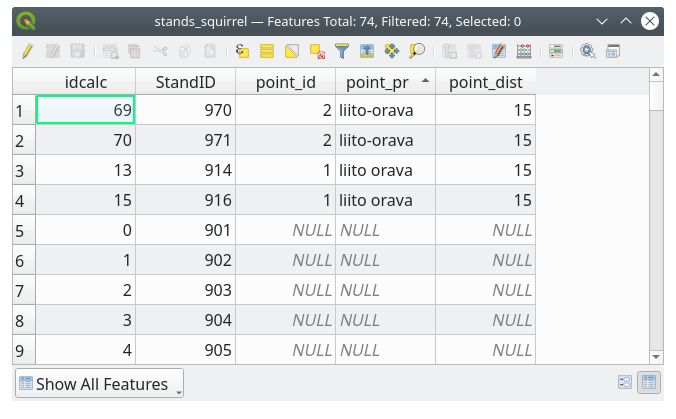
   You can see that there are some forest stands that have the information about the protection locations. The information in the forest stands data will indicate to the forest manager that there are protection considerations to be taken into account. Then he or she can get the location from the squirrel dataset, and visit the area to mark the corresponding buffer around the location so that the operators in the field can avoid disturbing the squirrels environment.

14.4.5. ★☆☆ Try Yourself: Updating Forest Stands with Distance to the Stream

Following the same approach as for the protected squirrel locations you can now update your forest stands with protection information related to the stream. A few points:

• Remember the buffer is 20 meters around the stream

• You want to have all the protection information in the same vector file, so use stands_squirrel.shp as the base layer

• Name your output as forest_stands_2012_protect.shp

Once the process is completed, open the attribute table of the output layer and confirm that you have all the protection information for the riparian forest stands associated with the stream.

When you are happy with the results, save your QGIS project.

14.4.6. Conclusion

Vous avez vu comment interprétez des images CIR pour numériser des massifs forestiers. Bien sûr cela demanderait plus de pratique pour faire des massifs plus précis et le plus souvent avec d’autres informations, comme des cartes pédologiques donneraient de meilleurs résultats, mais vous savez désormais les bases pour ce type de tâche. Et l’ajout d’informations à partir de jeux de données s’est révélé être une tâche tout à fait banale.

14.4.7. La suite ?

Les massifs de forêt que vous avez numérisés seront utilisés pour la planification des opérations forestières dans l’avenir, mais vous avez besoin d’obtenir toujours plus d’informations sur la forêt. Dans la prochaine leçon, vous verrez comment planifier un ensemble de parcelles d’échantillonnage pour inventorier la zone forestière que vous venez de numériser, et obtenir l’estimation globale des paramètres de la forêt.