Importante
A tradução é um esforço comunitário você pode contribuir. Esta página está atualmente traduzida em 28.49%.
11.1. Abrir Dados
Como parte de um ecossistema de software de código aberto, o QGIS é baseado em diferentes bibliotecas que, combinadas com seus próprios provedores, oferecem capacidades para ler e muitas vezes escrevem vários formatos:
Vector data formats include GeoPackage, GML, GeoJSON, GPX, KML, Comma Separated Values, ESRI formats (Shapefile, Geodatabase…), MapInfo and MicroStation file formats, AutoCAD DWG/DXF, GRASS and many more… Read the complete list of supported vector formats.
Raster data formats include GeoTIFF, JPEG, ASCII Gridded XYZ, MBTiles, R or Idrisi rasters, GDAL Virtual, SRTM, Sentinel Data, ERDAS IMAGINE, ArcInfo Binary Grid, ArcInfo ASCII Grid, and many more… Read the complete list of supported raster formats.
Database formats include PostgreSQL, SQLite/SpatiaLite, Oracle, MS SQL Server, SAP HANA, MySQL…
Web map and data services (WM(T)S, WFS, WCS, CSW, XYZ tiles, ArcGIS services, …) are also handled by QGIS providers. See Working with OGC / ISO protocols for more information about some of these.
You can read supported files from archived folders and use QGIS native formats such as QML files (QML - O Formato de Arquivo de Estilo QGIS) and virtual and memory layers.
More than 80 vector and 140 raster formats are supported by GDAL and QGIS native providers.
Nota
Not all of the listed formats may work in QGIS for various reasons.
For example, some require external proprietary libraries, or the GDAL/OGR
installation of your OS may not have been built to support the format you
want to use. To see the list of available formats, run the command line
ogrinfo --formats (for vector) and gdalinfo --formats (for raster),
or check the menu in QGIS.
In QGIS, depending on the data format, there are different tools to open a
dataset, mainly available in the menu
or from the Manage Layers toolbar (enabled through
menu).
However, all these tools point to a unique dialog, the Data Source
Manager dialog, that you can open with the  Open Data Source Manager button, available on the Data Source
Manager Toolbar, or by pressing Ctrl+L.
The Data Source Manager dialog (Fig. 11.1)
offers a unified interface to open file-based data as well as databases or
web services supported by QGIS.
Open Data Source Manager button, available on the Data Source
Manager Toolbar, or by pressing Ctrl+L.
The Data Source Manager dialog (Fig. 11.1)
offers a unified interface to open file-based data as well as databases or
web services supported by QGIS.
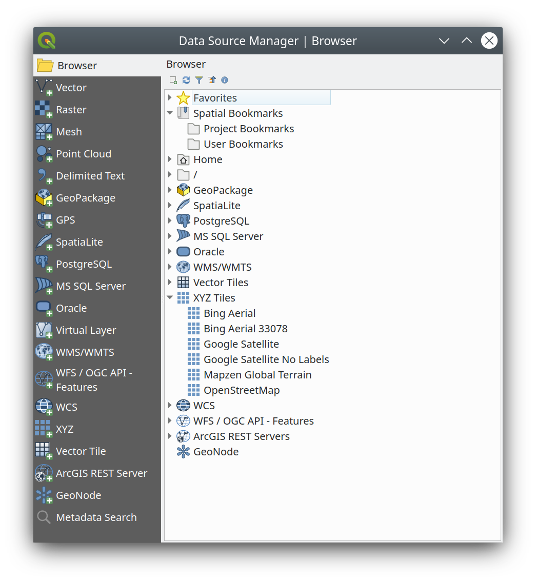
Fig. 11.1 QGIS Data Source Manager dialog
Beside this main entry point, you also have the  DB Manager plugin that offers advanced capabilities to analyze and
manipulate connected databases.
More information on DB Manager capabilities can be found in Plugin do gerenciador de banco de dados.
DB Manager plugin that offers advanced capabilities to analyze and
manipulate connected databases.
More information on DB Manager capabilities can be found in Plugin do gerenciador de banco de dados.
Existem muitas outras ferramentas, complementos nativos ou de terceiros, que ajudam a abrir vários formatos de dados.
Este capítulo descreve apenas as ferramentas fornecidas por padrão no QGIS para carregar dados. Ele se concentra principalmente na caixa de diálogo Gerenciador de Fonte de Dados, mas, além de descrever cada guia, também explora as ferramentas baseadas no provedor de dados ou nas especificidades do formato.
11.1.1. The Browser Panel
The Browser is one of the main ways to quickly and easily add your data to projects. It’s available as:
a Data Source Manager tab, enabled pressing the
Open Data Source Manager button (Ctrl+L);as a QGIS panel you can open from the menu (or
 ) or by pressing Ctrl+2.
In both cases, the Browser helps you navigate in your file system and manage geodata, regardless the type of layer (raster, vector, table), or the datasource format (plain or compressed files, databases, web services).
11.1.1.1. Explorando a Interface
Na parte superior do painel Navegador, você encontra alguns botões que ajudam a:
 Add Selected Layers: you can also add data to the map
canvas by selecting Add selected layer(s) from the layer’s context menu;
Add Selected Layers: you can also add data to the map
canvas by selecting Add selected layer(s) from the layer’s context menu; Refresh the browser tree;
 Filter Browser to search for specific data. Enter a search
word or wildcard and the browser will filter the tree to only show paths to
matching DB tables, filenames or folders – other data or folders won’t be
displayed. See the Browser Panel(2) example in Fig. 11.2.
The comparison can be case-sensitive or not. It can also be set to:
Filter Browser to search for specific data. Enter a search
word or wildcard and the browser will filter the tree to only show paths to
matching DB tables, filenames or folders – other data or folders won’t be
displayed. See the Browser Panel(2) example in Fig. 11.2.
The comparison can be case-sensitive or not. It can also be set to:Normal: mostra itens que contêm o texto de pesquisa
Wildcard(s): fine tune the search using the
?and/or*characters to specify the position of the search textExpressão regular
 Collapse All the whole tree;
 Enable/disable properties widget: when toggled on,
a new widget is added at the bottom of the panel showing, if applicable,
metadata for the selected item.
Enable/disable properties widget: when toggled on,
a new widget is added at the bottom of the panel showing, if applicable,
metadata for the selected item.
The entries in the Browser panel are organised hierarchically, and there are several top level entries:
Favorites where you can place shortcuts to often used locations
Spatial Bookmarks where you can store often used map extents (see Bookmarking extents on the map)
Project Home: for a quick access to the folder in which (most of) the data related to your project are stored. The default value is the directory where your project file resides.
Home directory in the file system and the filesystem root directory.
Connected local or network drives
Em seguida, vêm vários tipos de contêiner/banco de dados e protocolos de serviço, dependendo da sua plataforma e bibliotecas subjacentes:
 GeoPackage
 SpatiaLite
 PostgreSQL
 SAP HANA
 MS SQL Server
 Oracle
 WMS/WMTS
 Vector Tiles
 XYZ Tiles
 WCS
WCS WFS/OGC API-Features
 ArcGIS REST Server
11.1.1.2. Interacting with the Browser items
The browser supports drag and drop within the browser, from the browser to the canvas and Layers panel, and from the Layers panel to layer containers (e.g. GeoPackage) in the browser.
Project file items inside the browser can be expanded, showing the full layer tree (including groups) contained within that project. Project items are treated the same way as any other item in the browser, so they can be dragged and dropped within the browser (for example to copy a layer item to a geopackage file) or added to the current project through drag and drop or double click.
The context menu for an element in the Browser panel is opened by right-clicking on it.
Para entradas de diretório do sistema de arquivos, o menu de contexto oferece o seguinte:
to create in the selected entry a:
Diretório…
GeoPackage…
ShapeFile…
Add as a Favorite: favorite folders can be renamed (Rename favorite…) or removed (Remove favorite) any time.
Hide from Browser: hidden folders can be toggled to visible from the setting
Fast Scan this Directory
Abrir Diretório
Abrir no Terminal
Propriedades…
Propriedades do diretório…
For leaf entries that can act as layers in the project, the context menu will have supporting entries. For example, for non-database, non-service-based vector, raster and mesh data sources:
Adicionar camada ao projeto
Propriedades da Camada
Open with Data Source Manager…
ou Deletar “<name of file>”…
Mostrar em arquivos
Propriedades do arquivo
In the Layer properties entry, you will find (similar to what you will find in the vector and raster layer properties once the layers have been added to the project):
Metadados for the layer. para a camada. Grupos de Metadados: Informações do provedor (se possível,será um hiperlink para a fonte Path), Identificação, Extensão, Acesso, Campos (para camadas vetoriais), Bandas (para camadas raster), Contatos, Links (para camadas vetoriais), Referências (para camadas raster), Histórico.
A Preview panel
The attribute table for vector sources (in the Attributes panel).
Use Open with Data Source Manager… to directly open and configure the data source in the Data Source Manager using the URI of your data source. This simplifies the process of adding a layer from the Browser by allowing you to set specific opening options for the data source. It is currently available for vector (including the dedicated GeoPackage entry), raster, and SpatiaLite data sources.
Para adicionar uma camada ao projeto usando a Navegador:
Enable the Browser as described above. A browser tree with your file system, databases and web services is displayed. You may need to connect databases and web services before they appear (see dedicated sections).
Encontre a camada na lista.
Use the context menu, double-click its name, or drag-and-drop it into the map canvas. Your layer is now added to the Layers panel and can be viewed on the map canvas.
Dica
Abra um projeto QGIS diretamente do navegador
You can also open a QGIS project directly from the Browser panel by double-clicking its name or by drag-and-drop into the map canvas.
Depois que um arquivo é carregado, você pode ampliar usando as ferramentas de navegação do mapa. Para alterar o estilo de uma camada, abra a caixa de diálogo :guilabel: Propriedades da Camada clicando duas vezes no nome da camada ou clicando com o botão direito do mouse no nome da legenda e escolhendo :menuselection:` Propriedades` no menu de contexto. Veja a seção Propriedades da simbologia para mais informações sobre a configuração de simbologia para camadas vetoriais.
Right-clicking an item in the browser tree helps you to:
for a file or a table, display its metadata or open it in your project. Tables can even be renamed, deleted or truncated.
para uma pasta, adicione-a aos favoritos ou oculte-a na árvore do navegador. As pastas ocultas podem ser gerenciadas a partir da guia .
manage your spatial bookmarks: bookmarks can be created, exported and imported as
XMLfiles.crie uma conexão com um banco de dados ou um serviço da web.
atualizar, renomear ou excluir um esquema.
Você também pode importar arquivos para bancos de dados ou copiar tabelas de um esquema/banco de dados para outro com um simples arrastar e soltar. Há um segundo painel do navegador disponível para evitar rolagem longa enquanto arrasta. Basta selecionar o arquivo e arrastar e soltar de um painel para o outro.
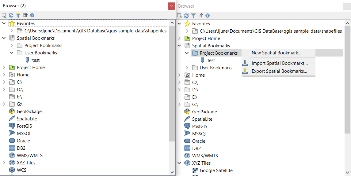
Fig. 11.2 QGIS Browser panels side-by-side
Dica
Add layers to QGIS by simple drag-and-drop from your OS file browser
You can also add file(s) to the project by drag-and-dropping them from your operating system file browser to the Layers Panel or the map canvas.
11.1.2. The DB Manager
The DB Manager Plugin is another tool for integrating and managing spatial database formats supported by QGIS (PostgreSQL, SpatiaLite, GeoPackage, Oracle Spatial, MS SQL Server, Virtual layers). It can be activated from the menu.
The DB Manager Plugin provides several features:
connect to databases and display their structure and contents
preview tables of databases
add layers to the map canvas, either by double-clicking or drag-and-drop.
add layers to a database from the QGIS Browser or from another database
create SQL queries and add their output to the map canvas
criar virtual layers
More information on DB Manager capabilities is found in Plugin do gerenciador de banco de dados.
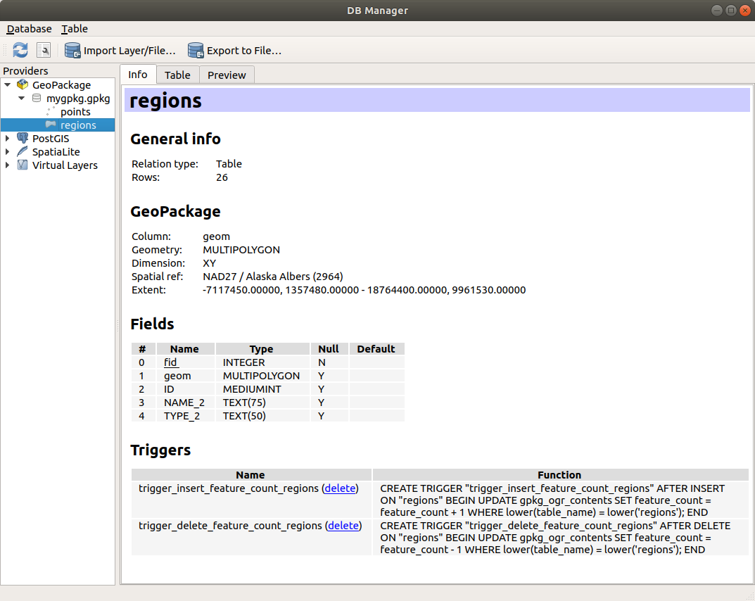
Fig. 11.3 Caixa de diálogo Gerenciador DB
11.1.3. Provider-based loading tools
Beside the Browser Panel and the DB Manager, the main tools provided by QGIS to add layers, you’ll also find tools that are specific to data providers.
Nota
Alguns: ‘plugins externos <plugins>’ também fornecem ferramentas para abrir arquivos de formato específico no QGIS.
11.1.3.1. Carregando uma camada de um arquivo
Para carregar uma camada de um arquivo:
Abra a guia do tipo de camada na caixa de diálogo Gerenciador de Fonte de Dados, ou seja, clique no botão
Abrir Gerenciador de Fonte de Dados (ou pressione: kbd:Ctrl+L) e ative a guia de destino ou:for vector data (like GML, ESRI Shapefile, Mapinfo and DXF layers): press Ctrl+Shift+V, select the
 Add Vector Layer menu option or
click on the Add Vector Layer toolbar button.
Add Vector Layer menu option or
click on the Add Vector Layer toolbar button.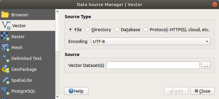
Fig. 11.4 Add Vector Layer Dialog
para dados raster (como camadas GeoTiff, MBTiles, GRIdded Binary e DWG): pressione Ctrl+Shift+R, selecione a opção
 Adicionar Camada Raster do menu ou clique no botão Adicionar Camada Raster da barra de ferramentas.
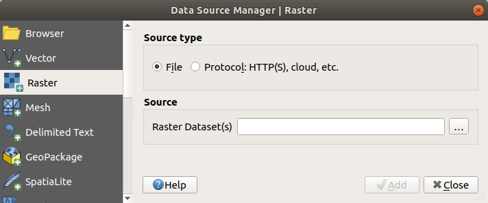
Fig. 11.5 Add Raster Layer Dialog
Check
 File source type
Click on the … Browse button
Navegue no sistema de arquivos e carregue uma fonte de dados suportada. É possível carregar mais de uma camada ao mesmo tempo mantendo pressionada a tecla Ctrl e clicando em vários itens da caixa de diálogo ou pressionando a tecla Shift para selecionar um intervalo de itens clicando em o primeiro e o último item do intervalo. Somente os formatos que foram bem testados aparecem no filtro de formatos. Outros formatos podem ser carregados selecionando
Todos os arquivos(o item superior no menu pull-down).Press Open to load the selected file into Data Source Manager dialog.
Depending on the selected layer type, additional Options (encoding, geometry type, table filtering, file locking, data formatting …) are available for configuring. These options are described in detail in the specific GDAL vector or raster driver documentation. At the top of the options, a text with hyperlink will directly lead to the documentation of the appropriate driver for the selected file format.
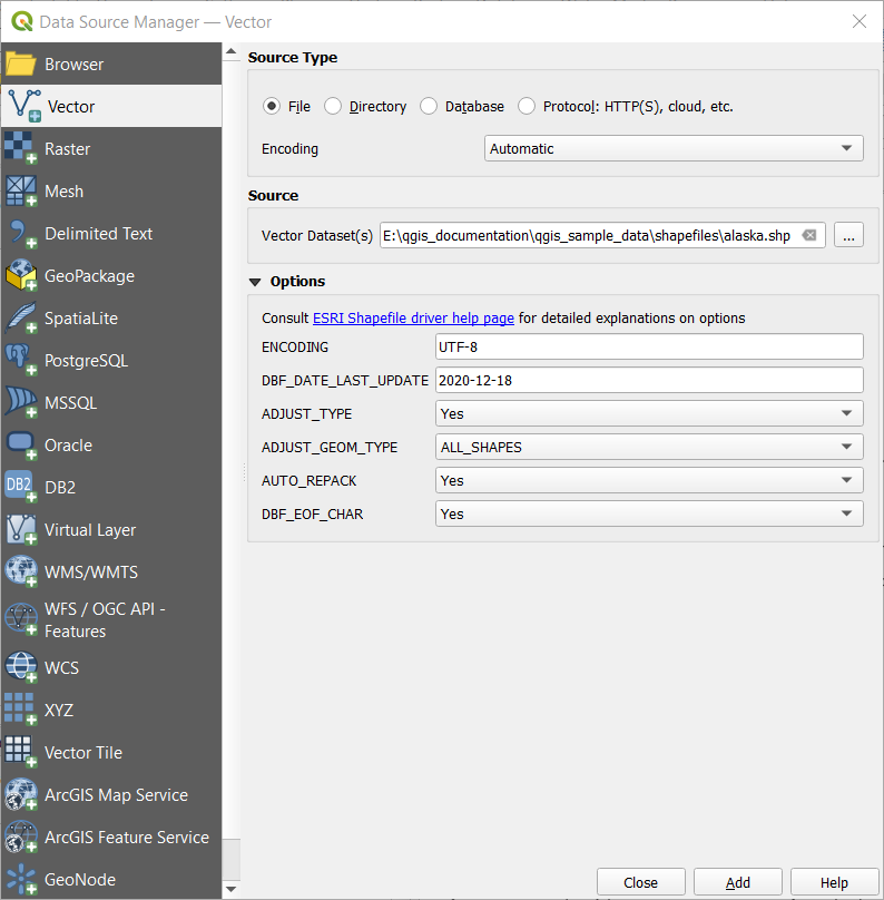
Fig. 11.6 Carregando um Shapefile com opções em aberto
Press Add to load the file in QGIS and display them in the map view. When adding vector datasets containing multiple layers, the Select Items to Add dialog will appear. In this dialog, you can choose the specific layers from your dataset that you want to add. Also, under Options you can choose to:
 Add layers to a group
- Show system and internal tables
- Show empty vector layers.
Fig. 11.7 shows QGIS after loading the
alaska.shpfile.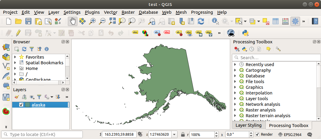
Fig. 11.7 QGIS com Shapefile do Alasca carregado
Nota
Como alguns formatos como MapInfo (por exemplo, .tab) ou Autocad (.dxf) permitem misturar diferentes tipos de geometria em um único arquivo, carregar tais conjuntos de dados abre um diálogo para selecionar as geometrias a serem utilizadas a fim de ter uma geometria por camada.
The Add Vector Layer and Add Raster
Layer tabs allow loading of layers from source types other than File:
You can load specific vector formats like
ArcInfo Binary Coverage,UK. National Transfer Format, as well as the raw TIGER format of theUS Census BureauorOpenfileGDB. To do that, you select Directory as Source type.
In this case, a directory can be selected in the dialog after pressing
… Browse.With the
Database source type you can select an
existing database connection or create one to the selected database type.
Some possible database types are ODBC,Esri Personal Geodatabase,MS SQL Serveras well asPostgreSQLorMySQL.Pressing the New button opens the Create a New OGR Database Connection dialog whose parameters are among the ones you can find in Criando uma conexão armazenada. Pressing Open lets you select from the available tables.
O tipo de fonte
Protocolo: HTTP(S), nuvem, etc. abre dados armazenados localmente ou na rede sejam publicamente acessíveis, ou em armazenamentos em nuvem particulares fornecidos por serviços comerciais. Os tipos de protocolo suportados são:HTTP/HTTPS/FTP, with a URI and, if required, an authentication.Cloud storage such as
AWS S3,Google Cloud Storage,Microsoft Azure Blob,Microsoft Azure Data Lake Storage,Alibaba OSS Cloud, andOpen Stack Swift Storagesupports direct control over VSI Credential Options when adding OGR vector or GDAL raster layers. You need to fill in the Bucket or container and the Object key first. After that, you can add the necessary Credential Options.When adding OGR vector or GDAL raster layers from the cloud based protocols, you can also set additional Credential options for that specific driver and bucket. When credential options are found in a layer’s URI, they will also be automatically set. This allows different layers to use different credentials.
service supporting OGC
WFS 3(still experimental), usingGeoJSONorGEOJSON - Newline Delimitedformat or based onCouchDBdatabase. A URI is required, with optional authentication.For all vector source types it is possible to define the Encoding or to use the setting.
The
OGC API source type allows you to access
vector
and raster data
from servers that implement the OGC API standards.
To use this option:Select
OGC API from the Data Source Manager
dialog.Enter the endpoint of the OGC API service you want to connect to. Note that you don’t need to prefix the endpoint with “OGCAPI:”.
Click Connect to establish a connection to the server.
11.1.3.2. Carregando uma camada de malha
A mesh is an unstructured grid usually with temporal and other components. The spatial component contains a collection of vertices, edges and faces in 2D or 3D space. More information on mesh layers at Working with Mesh Data.
Para adicionar uma camada de malha ao QGIS:
Open the dialog, either by selecting it from the menu or clicking the
Open Data Source Manager button.Ative a guia
 Malha no painel da esquerda
Pressione o botão … Buscar para selecionar o arquivo. Vários formatos são suportados.
Select the file and press Add. The layer will be added using the native mesh rendering.
If the selected file contains many mesh layers, then you’ll be prompted with a dialog to choose the sublayers to load. Do your selection and press OK and the layers are loaded with the native mesh rendering. It’s also possible to load them within a group.
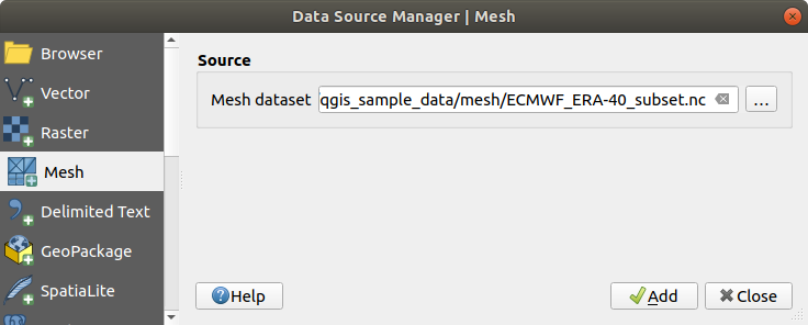
Fig. 11.8 Mesh tab in Data Source Manager
11.1.3.3. Importando um arquivo de texto delimitado
Delimited text files (e.g. .txt, .csv, .dat,
.wkt) can be loaded using the tools described above.
This way, they will show up as simple tables.
Sometimes, delimited text files can contain coordinates / geometries
that you could want to visualize.
This is what  Add Delimited Text Layer
is designed for.
Add Delimited Text Layer
is designed for.
Click the
Open Data Source Manager icon to
open the Data Source Manager dialogAtive a guia
Texto DelimitadoSelect the delimited text file to import (e.g.,
qgis_sample_data/csv/elevp.csv) by clicking on the … Browse button.Configure as configurações para atender seu conjunto de dados e necessidades, conforme explicado abaixo.
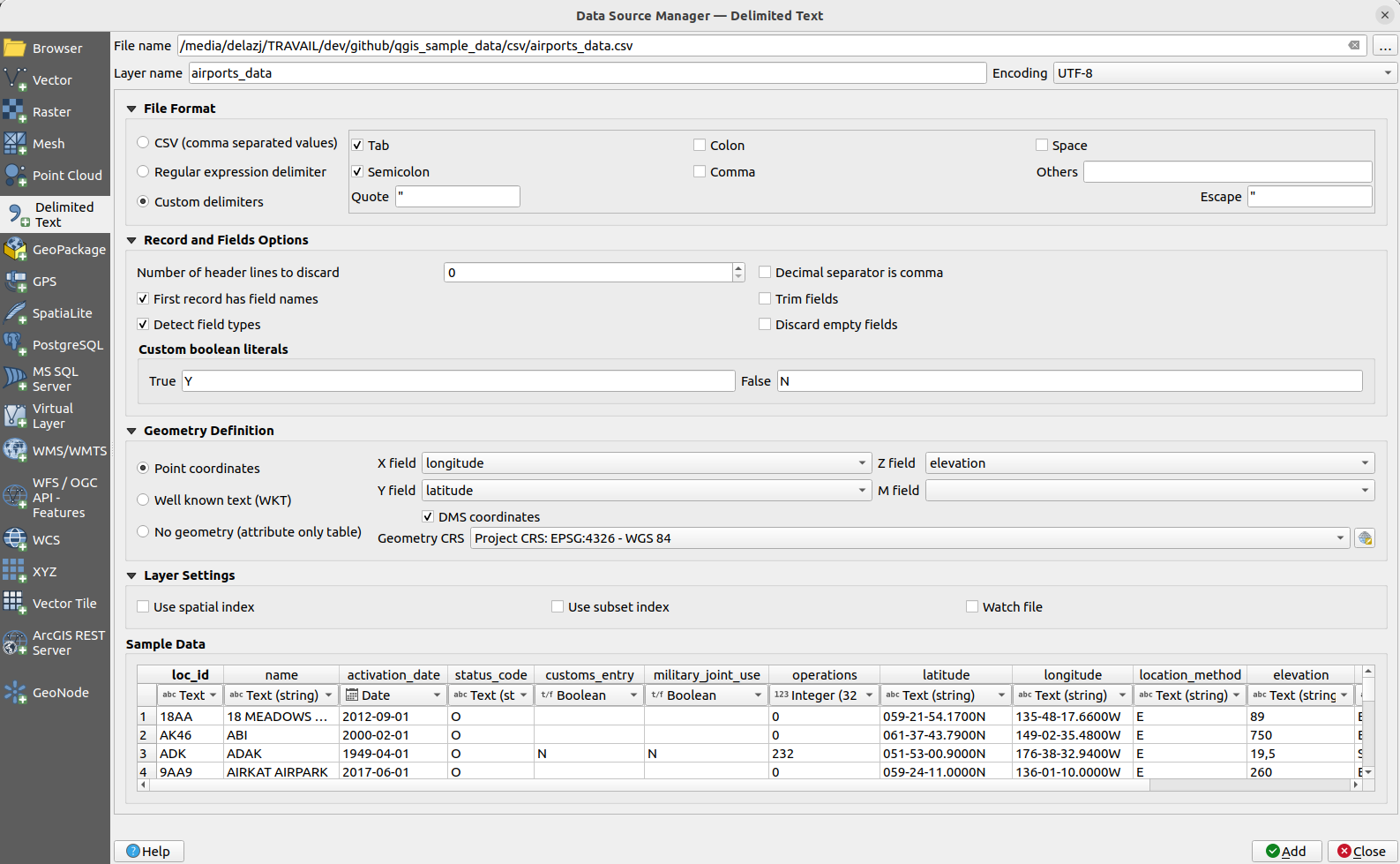
Fig. 11.9 Delimited Text Dialog
Formato de arquivo
Depois que o arquivo é selecionado, o QGIS tenta analisar o arquivo com o delimitador usado mais recentemente, identificando campos e linhas. Para permitir que o QGIS analise corretamente o arquivo, é importante selecionar o delimitador correto. Você pode especificar um delimitador escolhendo entre:
- CSV (valores separados por vírgula) para utilizar o caractere de vírgula.
 Regular expression delimiter and enter text
into the Expression field.
For example, to change the delimiter to tab, use
Regular expression delimiter and enter text
into the Expression field.
For example, to change the delimiter to tab, use \t(this is used in regular expressions for the tab character).- Custom delimiters, choosing among some predefined
delimiters like
comma,space,tab,semicolon, … .
Registros e campos
Algumas outras opções convenientes podem ser usadas para reconhecimento de dados:
Number of header lines to discard: convenient when you want to avoid the first lines in the file in the import, either because those are blank lines or with another formatting.
- First record has field names: values in the first
line are used as field names, otherwise QGIS uses the field names
field_1,field_2… - Detect field types: automatically recognizes the field
type. If unchecked then all attributes are treated as text fields.
- Separador decimal é vírgula: você pode forçar o separador decimal a ser uma vírgula.
- Trim fields: allows you to trim leading and trailing
spaces from fields.
- Discard empty fields.
Custom boolean literals: allows you to add a custom couple of string that will be detected as boolean values.
Field type detection
QGIS tries to detect the field types automatically (unless
Detect field types is not checked) by examining
the content of an optional sidecar CSVT file (see GeoCSV specification)
and by scanning the whole file to make sure that all values can actually
be converted without errors, the fall-back field type is text.
The detected field type appears under the field name in sample data preview table and can be manually changed if necessary.
The following field types are supported:
Booleancase-insensitive literal couples that are interpreted as boolean values are1/0,true/false,t/f,yes/noWhole Number (integer)Whole Number (integer - 64 bit)Decimal Number: double precision floating point numberDateTimeDate and TimeText
Definição de geometria
Once the file is parsed, set Geometry definition to
- Point coordinates and provide the X
field, Y field, Z field (for 3-dimensional data)
and M field (for the measurement dimension) if the layer is of
point geometry type and contains such fields. If the coordinates
are defined as degrees/minutes/seconds, activate the
DMS coordinates checkbox.
Provide the appropriate Geometry CRS using the
 Select CRS widget.
 - Well known text (WKT) option if the spatial
information is represented as WKT: select the Geometry field
containing the WKT geometry and choose the appropriate Geometry
field or let QGIS auto-detect it.
Provide the appropriate Geometry CRS using the
Select CRS widget.
If the file contains non-spatial data, activate
No
geometry (attribute only table) and it will be loaded as an ordinary table.
Configurações de camada
Além disso, você pode habilitar:
- Use spatial index to improve the performance of
displaying and spatially selecting features.
- Use subset index to improve performance of subset
filters (when defined in the layer properties).
- Watch file to watch for changes to the file by other
applications while QGIS is running.
At the end, click Add to add the layer to the map.
In our example, a point layer named Elevation is added to the project
and behaves like any other map layer in QGIS.
This layer is the result of a query on the .csv source file
(hence, linked to it) and would require
to be saved in order to get a spatial layer on disk.
Sample Data
As you set the parser properties, the sample data preview updates regarding to the applied settings.
Also in the Sample Data Table it is possible to override the automatically determined column types.
11.1.3.4. Importando um arquivo DXF ou DWG
DXF and DWG files can be added to QGIS by simple drag-and-drop
from the Browser Panel.
You will be prompted to select the sublayers you would like to add
to the project. Layers are added with random style properties.
Nota
For DXF files containing several geometry types (point, line and/or polygon), the name of the layers will be generated as <filename.dxf> entities <geometry type>.
To keep the dxf/dwg file structure and its symbology in QGIS, you may want to use the dedicated tool which allows you to:
import elements from the drawing file into a GeoPackage database.
adicionar elementos importados ao projeto.
In the DWG/DXF Import dialog, to import the drawing file contents:
Input the location of the Source drawing, i.e. the DWG/DXF drawing file to import.
Especifique o sistema de referência de coordenadas dos dados no arquivo de desenho.
Input the location of the Target package, i.e. the GeoPackage file that will store the data. If an existing file is provided, then it will be overwritten.
Choose how to import
blockswith the dedicated combobox:Expand Block Geometries: imports the blocks in the drawing file as normal elements.
Expand Block Geometries and Add Insert Points: imports the blocks in the drawing file as normal elements and adds the insertion point as a point layer.
Add Only Insert Points: adds the blocks insertion point as a point layer.
Check
Use curves to promote the imported layers
to a curvedgeometry type.Use the Import button to import the drawing into the destination GeoPackage file. The GeoPackage database will be automatically populated with the drawing file content. Depending on the size of the file, this can take some time.
After the .dwg or .dxf data has been imported into the
GeoPackage database, the frame in the lower half of the dialog is
populated with the list of layers from the imported file.
There you can select which layers to add to the QGIS project:
At the top, set a Group name to group the drawing files in the project. By default this is set to the filename of the source drawing file.
Check layers to show: Each selected layer is added to an ad hoc group which contains vector layers for the point, line, label and area features of the drawing layer. The style of the layers will resemble the look they originally had in *CAD.
Escolha se a camada deve estar visível na abertura.
Marcar a opção
Mesclar camadas coloca todas as camadas em um único grupo.Press OK to open the layers in QGIS.
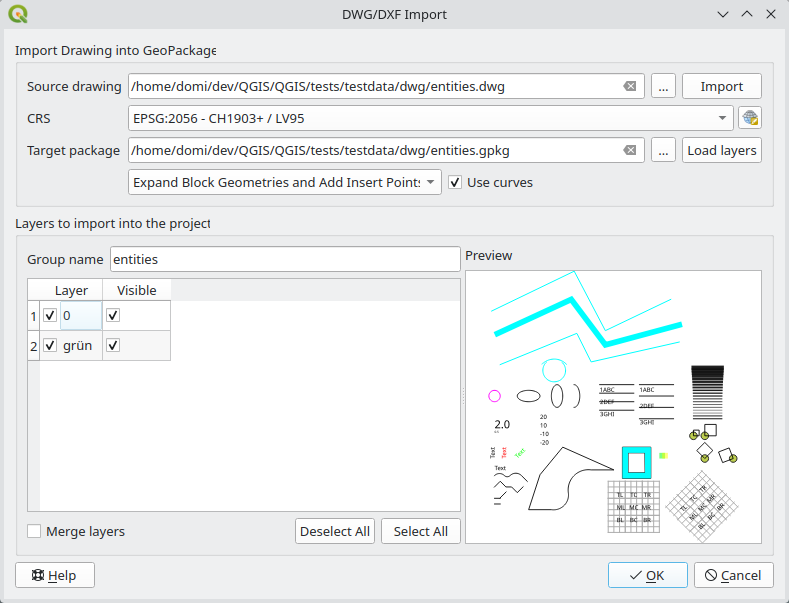
Fig. 11.10 Import dialog for DWG/DXF files
11.1.3.5. Importando vetores OpenStreetMap
The OpenStreetMap project is popular because in many countries no free geodata such as digital road maps are available. The objective of the OSM project is to create a free editable map of the world from GPS data, aerial photography and local knowledge. To support this objective, QGIS provides support for OSM data.
Using the Browser Panel, you can load an .osm file to the
map canvas, in which case you’ll get a dialog to select sublayers based on the
geometry type.
The loaded layers will contain all the data of that geometry type
in the .osm file, and keep the osm file data structure.
11.1.3.6. Camadas SpatiaLite
 The first time you load data from a SpatiaLite
database, begin by:
The first time you load data from a SpatiaLite
database, begin by:
clicking on the
Add SpatiaLite Layer toolbar
buttonselecting the
option from the menuou digitando Ctrl+Shift+L
This will bring up a window that will allow you either to connect to a
SpatiaLite database already known to QGIS (which you choose from the
drop-down menu) or to define a new connection to a new database. To define a
new connection, click on New and use the file browser to point to
your SpatiaLite database, which is a file with a .sqlite extension.
O QGIS também suporta visualizações editáveis no SpatiaLite.
11.1.3.7. GPS
Existem dezenas de formatos de arquivo diferentes para armazenar dados GPS. O formato que o QGIS usa é chamado GPX (formato GPS eXchange), que é um formato padrão de intercâmbio que pode conter qualquer número de pontos de passagem, rotas e trilhas no mesmo arquivo.
Use the … Browse button to select the GPX file, then use the check boxes to select the feature types you want to load from that GPX file. Each feature type will be loaded in a separate layer.
More on GPS data manipulation at Trabalhando com dados GPS.
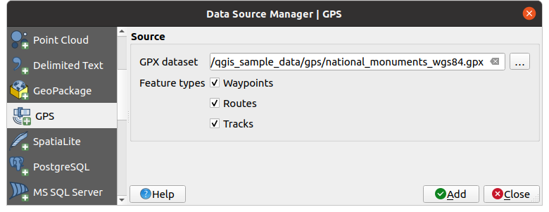
Fig. 11.11 Carregando a janela de dados do GPS
11.1.3.8. GRASS
Working with GRASS vector data is described in section Integração com SIG GRASS.
11.1.3.9. Database related tools
Criando uma conexão armazenada
In order to read and write tables from a database format QGIS supports you have to create a connection to that database. While QGIS Browser Panel is the simplest and recommended way to connect to and use databases, QGIS provides other tools to connect to each of them and load their tables:
 or by typing
Ctrl+Shift+D
or by typing
Ctrl+Shift+D or by typing
Ctrl+Shift+O
or by typing
Ctrl+Shift+O
 or by typing
Ctrl+Shift+G
or by typing
Ctrl+Shift+G
These tools are accessible either from the Manage Layers Toolbar and the menu. Connecting to SpatiaLite database is described at Camadas SpatiaLite.
Dica
Create connection to database from the QGIS Browser Panel
Selecting the corresponding database format in the Browser tree, right-clicking and choosing connect will provide you with the database connection dialog.
Most of the connection dialogs follow a common structure:
a section with credentials information to connect to the database
a section with options to tune which data can be requested in the database
Connecting to PostgreSQL
The first time you use a PostgreSQL data source, you must create a connection to a database that contains the data. Press the appropriate button as exposed above, opening the PostgreSQL tab of the Data Source Manager dialog. To access the connection manager, click on the New button to display the Create a New PostgreSQL Connection dialog.
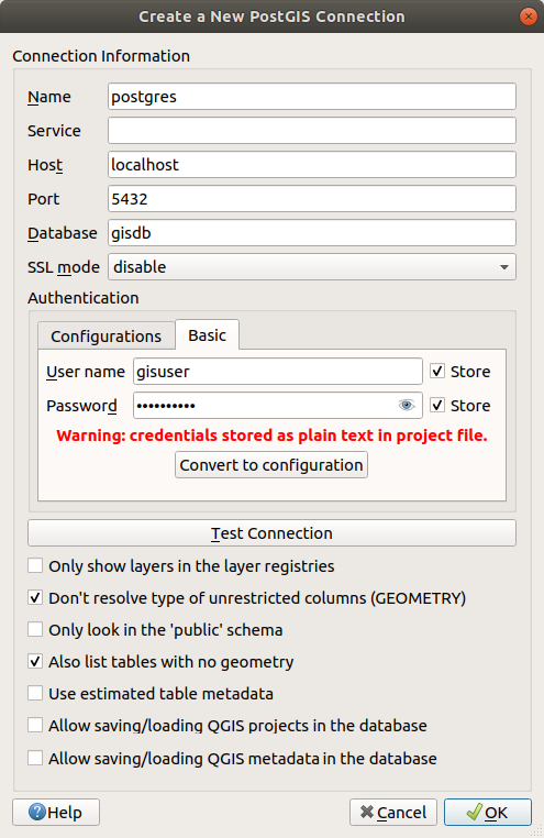
Fig. 11.12 Create a New PostgreSQL Connection Dialog
Name: A name for this connection. It can be the same as Database.
Service: Service parameter to be used alternatively to hostname/port (and potentially database). This can be defined in
pg_service.conf. Check the PostgreSQL Service connection file section for more details.Host: Name of the database host. This must be a resolvable host name such as would be used to open a TCP/IP connection or ping the host. If the database is on the same computer as QGIS, simply enter localhost here.
Port: Port number the PostgreSQL database server listens on. The default port for PostgreSQL is
5432.Banco de Dados: Nome do banco de dados.
SSL mode: SSL encryption setup. The following options are available:
Prefer (the default): I don’t care about encryption, but I wish to pay the overhead of encryption if the server supports it.
Require: I want my data to be encrypted, and I accept the overhead. I trust that the network will make sure I always connect to the server I want.
Verify CA: I want my data encrypted, and I accept the overhead. I want to be sure that I connect to a server that I trust.
Guilabel: ‘Verificação Completa’: Quero meus dados criptografados, e aceito as despesas gerais. Quero ter certeza de que me conecto a um servidor em que confio, e que é aquele que eu especifico.
guilabel: ‘Permitir’: Eu não me importo com a segurança, mas pagarei as despesas gerais de criptografia se o servidor insistir nisso.
guilabel:`Desativar’: Eu não me importo com a segurança, e não quero pagar as despesas gerais de criptografia.
Session role: used to set the current user identifier of the current session. This is useful to automatically give the ownership of a new object (table, view, function) to the session_role group and thus share ownership and associated rights with all members of the session_role group. Read more about session role.
Authentication: For general details about the authentication dialog behavior, see Autenticação.
Opcionalmente, dependendo do tipo de banco de dados, você pode ativar as seguintes caixas de seleção:
- Only show layers in the layer registries
- :guilabel:`Não resolva o tipo de colunas irrestritas (GEOMETRIA) `
- Also list tables with no geometry:
indicates that tables without geometry should also be listed by default.
- Use estimated table metadata: When initializing layers,
various queries may be needed to establish the characteristics of the geometries
stored in the database table.
When this option is checked, these queries examine only a sample of the rows
and use the table statistics, rather than the entire table.
This can drastically speed up operations on large datasets,
but may result in incorrect characterization of layers
(e.g. the feature count of filtered layers will not be accurately determined)
and may even cause strange behaviour if columns that are supposed to be unique
actually are not.
- Permitir salvar/carregar projetos QGIS no banco de dados - mais detalhes here
- Allow saving/loading QGIS layer metadata in the database
- more details here
- Also list raster overview tables
- Only look in the ‘public’ schema
Schema: Allows to specify a single schema to limit a connection to. When set, only tables from the matching schema will be included in the browser panel and data source select for the connection. This can be used to limit the database work required to populate tables for a connection pointing to a large database store.
Once all parameters and options are set, you can test the connection by clicking the Test Connection button or apply it by clicking the OK button.
PostgreSQL Service connection file
The service connection file allows PostgreSQL connection parameters to be associated with a single service name. That service name can then be specified by a client and the associated settings will be used.
It’s called .pg_service.conf under *nix systems (GNU/Linux, macOS etc.)
and pg_service.conf on Windows.
O arquivo de serviço pode se parecer com o seguinte:
[water_service]
host=192.168.0.45
port=5433
dbname=gisdb
user=paul
password=paulspass
[wastewater_service]
host=dbserver.com
dbname=water
user=waterpass
Nota
There are two services in the above example: water_service
and wastewater_service. You can use these to connect from QGIS,
pgAdmin, etc. by specifying only the name of the service you want to
connect to (without the enclosing brackets).
If you want to use the service with psql, you can do psql service=water_service.
You can find all the PostgreSQL parameters here
Nota
If you don’t want to save the passwords in the service file you can use the .pg_pass option.
Nota
QGIS Server and service
When using a service file and QGIS Server, you must configure the service on the server side as well. You can follow the QGIS Server documentation.
On *nix operating systems (GNU/Linux, macOS etc.) you can save the
.pg_service.conf file in the user’s home directory and
PostgreSQL clients will automatically be aware of it.
For example, if the logged user is web, .pg_service.conf should
be saved in the /home/web/ directory in order to directly work (without
specifying any other environment variables).
You can specify the location of the service file by creating a
PGSERVICEFILE environment variable (e.g. run the
export PGSERVICEFILE=/home/web/.pg_service.conf
command under your *nix OS to temporarily set the PGSERVICEFILE variable).
You can also make the service file available system-wide (all users) either by
placing the .pg_service.conf file in pg_config --sysconfdir or by
adding the PGSYSCONFDIR environment variable to specify the directory
containing the service file. If service definitions with the same name exist
in the user and the system file, the user file takes precedence.
Aviso
There are some caveats under Windows:
The service file should be saved as
pg_service.confand not as.pg_service.conf.The service file should be saved in Unix format in order to work. One way to do it is to open it with Notepad++ and .
Você pode adicionar variáveis ambientais de várias maneiras; um testado, conhecido por funcionar de forma confiável, é :menuelection:`Painel de controle --> Sistema e segurança --> Sistema --> Configurações avançadas do sistema --> Variáveis de ambiente` adicionando
PGSERVICEFILEcom o caminho - por exemploC:\Users\John\pg_service.confAfter adding an environment variable you may also need to restart the computer.
Conectando ao Oracle Spatial

Fig. 11.13 Create a New Oracle Connection Dialog
The spatial features in Oracle Spatial aid users in managing geographic and location data in a native type within an Oracle database. The connection dialog proposes:
Name: A name for this connection. It can be the same as Database;
Database: SID or SERVICE_NAME of the Oracle instance;
Host: The name of the database host;
Port: Port number the Oracle database server listens on. The default port is
1521;Options: Oracle connection specific options (e.g. OCI_ATTR_PREFETCH_ROWS, OCI_ATTR_PREFETCH_MEMORY). The format of the options string is a semicolon separated list of option names or option=value pairs;
Workspace: Workspace to switch to;
Authentication: For general details about the authentication dialog behavior, see Autenticação.
Opcionalmente, você pode ativar as seguintes caixas de seleção:
- Only look in metadata table: restricts the displayed
tables to those that are in the
all_sdo_geom_metadataview. This can speed up the initial display of spatial tables. - Only look for user’s tables: when searching for spatial tables,
restricts the search to tables that are owned by the user.
- Also list tables with no geometry:
indicates that tables without geometry should also be listed by default.
- Use estatísticas estimadas da tabela para os metadados da camada: quando a camada é configurada, vários metadados são necessários para a tabela Oracle. Isso inclui informações como a contagem de linhas da tabela, tipo de geometria e extensões espaciais dos dados na coluna geometria. Se a tabela contiver um grande número de linhas, a determinação desses metadados poderá ser demorada. Ao ativar esta opção, as seguintes operações rápidas de metadados da tabela são concluídas: A contagem de linhas é determinada em
all_tables.num_rows. As extensões de tabela são sempre determinadas com a função SDO_TUNE.EXTENTS_OF, mesmo se um filtro de camada for aplicado. A geometria da tabela é determinada a partir das primeiras 100 linhas de geometria não nula da tabela. - Only existing geometry types:
only lists the existing geometry types and don’t offer to add others.
- Permitir salvar/carregar projetos QGIS no banco de dados - mais detalhes here
Schema: Allows to specify a single schema to limit a connection to. When set, only tables from the matching schema will be included in the browser panel and data source select for the connection. This can be used to limit the database work required to populate tables for a connection pointing to a large database store.
Dica
Camadas Espaciais Oracle
Normally, an Oracle Spatial layer is defined by an entry in the USER_SDO_METADATA table.
To ensure that selection tools work correctly, it is recommended that your tables have a primary key.
Connecting to MS SQL Server
As mentioned in Criando uma conexão armazenada QGIS allows you to create MS SQL Server connection through Data Source Manager.
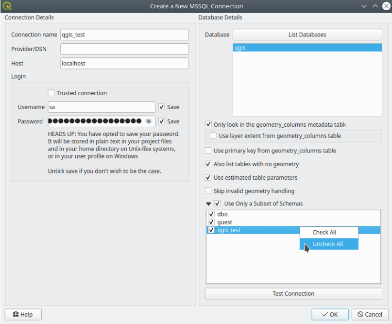
Fig. 11.14 MS SQL Server Connection
To create a new MS SQL Server connection, you need to provide some of the following information in the Connection Details dialog:
Connection name
Provider/DSN
Host
Login information. You can choose to
Save your credentials.
Navigate to the Database Details section and click the List Databases button to view the available datasets. Select datasets that you want, then press OK. Optionally, you can also perform a Test Connection. Once you click OK the Create a New MS SQL Server Connection dialog will close and in the Data Source Manager press Connect, select a layer and then click Add.
Optionally, you can activate the following options:
- Only look in the geometry_columns metadata table:
restricts the available tables to the ones in the
geometry_columnsmetadata table when scanning for tables. This can speed up the table scanning. - Use layer extent from geometry_columns table:
this option, dependent on the previous one, allows QGIS to skip extent calculation
when loading layers and thus lowering the amount of time needed to load them.
It relies on extent manually specified using additional QGIS-specific columns
(
qgis_xmin,qgis_xmax,qgis_ymin,qgis_ymax) in thegeometry_columnstable. - Use primary key from geometry_columns table:
allows QGIS to skip primary key calculation for views when loading them,
thus lowering the amount of time needed to load them.
It relies on names manually filled in a QGIS-specific
qgis_pkeycolumn set in thegeometry_columnstable. If more than one column is used for the primary key, they should be filled as comma separated values. - Also list table with no geometry: tables without a
geometry column attached will also be shown in the available table list.
- Use estimated table parameters: only estimated table
metadata will be used. This avoids a slow table scan, but may result in
incorrect layer properties such as layer extent.
- Skip invalid geometry handling: all handling of records
with invalid geometry will be disabled. This speeds up the provider, however,
if any invalid geometries are present in a table then the result is unpredictable
and may include missing records. Only check this option if you are certain that
all geometries present in the database are valid, and any newly added geometries
or tables will also be valid.
- Use only a Subset of Schemas will allow you to filter
schemas for MS SQL connection. If enabled, only checked schemas will be displayed.
You can right-click to Check or Uncheck any schema in the list.
Connecting to SAP HANA
Nota
You require the SAP HANA Client to connect to a SAP HANA database. You can download the SAP HANA Client for your platform at the SAP Development Tools website.
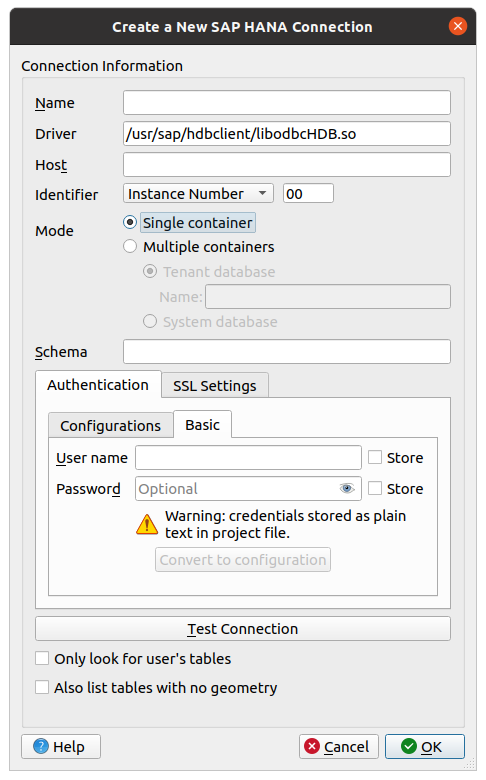
Fig. 11.15 Create a New SAP HANA Connection Dialog
Os seguintes parâmetros podem ser inseridos:
Nome: Um nome para esta conexão.
Driver
 : The name of the HANA ODBC driver. It is
 HDBODBCif you are using 64-bit QGIS,HDBODBC32if you are using 32-bit QGIS. The appropriate driver name is entered automatically.Driver

 : Either the name under which the SAP HANA ODBC
driver has been registered in
: Either the name under which the SAP HANA ODBC
driver has been registered in /etc/odbcinst.inior the full path to the SAP HANA ODBC driver. The SAP HANA Client installer will install the ODBC driver to/usr/sap/hdbclient/libodbcHDB.soby default.Host: The name of the database host.
Identifier: Identifies the instance to connect to on the host. This can be either Instance Number or Port Number. Instance numbers consist of two digits, port numbers are in the range from 1 to 65,535.
Mode: Specifies the mode in which the SAP HANA instance runs. This setting is only taken into account if Identifier is set to Instance Number. If the database hosts multiple containers, you can either connect to a tenant with the name given at Tenant database or you can connect to the system database.
Schema: This parameter is optional. If a schema name is given, QGIS will only search for data in that schema. If this field is left blank, QGIS will search for data in all schemas.
Authentication: For general details about the authentication dialog behavior, see Autenticação.
SSL Settings
- Enable TLS/SSL encryption: Enables TLS 1.1 - TLS1.2
encryption. The server will choose the highest available.
Provider: Specifies the cryptographic library provider used for SSL communication. sapcrypto should work on all platforms, openssl should work on
, mscrypto should
work on and commoncrypto requires CommonCryptoLib to be
installed.- Validate SSL certificate: If checked, the SSL
certificate will be validated using the truststore given in
Trust store file with public key.
Override hostname in certificate: Specifies the host name used to verify server’s identity. The host name specified here verifies the identity of the server instead of the host name with which the connection was established. If you specify
*as the host name, then the server’s host name is not validated. Other wildcards are not permitted.Keystore file with private key: Currently ignored. This parameter might allow to authenticate via certificate instead via user and password in future.
Trust store file with public key: Specifies the path to a trust store file that contains the server’s public certificates if using OpenSSL. Typically, the trust store contains the root certificate or the certificate of the certification authority that signed the server’s public certificates. If you are using the cryptographic library CommonCryptoLib or msCrypto, then leave this property empty.
- Only look for user’s tables: If checked, QGIS searches
only for tables and views that are owned by the user that connects to the
database.
- Use estimated table metadata: If checked, estimated
table metadata will be used if available. For large tables, this avoids slow
table loads and potentially expensive computations, but may result in
incorrect layer properties such as layer extent. The fast extent estimation
is available starting with QRC1/2024 and SP8 in HANA Cloud and HANA On-Premise
respectively.
- Also list tables with no geometries: If checked, QGIS
searches also for tables and views that do not contain a spatial column.
Dica
Connecting to SAP HANA Cloud
If you’d like to connect to an SAP HANA Cloud instance, you usually must set
Port Number to 443 and check
Enable TLS/SSL encryption.
Loading a Database Layer
Once you have one or more connections defined to a database (see section Criando uma conexão armazenada), you can load layers from it. Of course, this requires that data are available. See section Importing Data into PostgreSQL for a discussion on importing data into a PostgreSQL database.
Para carregar uma camada de um banco de dados, você pode executar as seguintes etapas:
Open the corresponding tab of the database in the Data Source Manager dialog.
Choose the connection name from the drop-down list and press Connect.
The table below will be filled with your data grouped by schema, with a number of metadata information helpful for loading.
Select or unselect
Also list tables with no geometry.Optionally, use some
Search Options to reduce the
list of tables to those matching your search. You can also set this option
before you hit the Connect button, speeding up the database
fetching.Encontre a(s) camada(s) que deseja adicionar na lista de camadas disponíveis.
Select it by clicking on it. You can select multiple layers by holding down the Shift or Ctrl key while clicking.
Layers can be selected only if they have no
 warning icon
at the left-hand side of their first column.
This may indicate an issue to detect:
warning icon
at the left-hand side of their first column.
This may indicate an issue to detect:features geometry type: in which case you can select the appropriate one in the drop-down list of the Spatial Type column
layer CRS: you can enter the correct code in the SRID column
layer’s primary key, in order to unequivocally identify each feature: this can be fixed by selecting one or more attributes in the drop-down list at the corresponding Feature id column.
Dica
Use the first column to store “primary keys” for views
Since PostgreSQL views don’t support primary keys, a unique attribute or combination of attributes should always be selected. To help users to speed-up workflows, QGIS automatically selects the first attribute in the view. Therefore, users can define their views in a way that a unique column is in the first position of the view’s definition. In this way, the view will be loaded with no extra interaction and the warning icon will never appear.
If applicable, use the Set Filter button (or double-click the layer) to start the Query Builder dialog (see section Criador de consultas) and define which features to load from the selected layer. The filter expression appears in the
sqlcolumn. This restriction can be removed or edited in the frame.The checkbox in the
Select at idcolumn that is activated by default gets the feature ids without the attributes and generally speeds up the data loading.Click on the Add button to add the layer to the map.
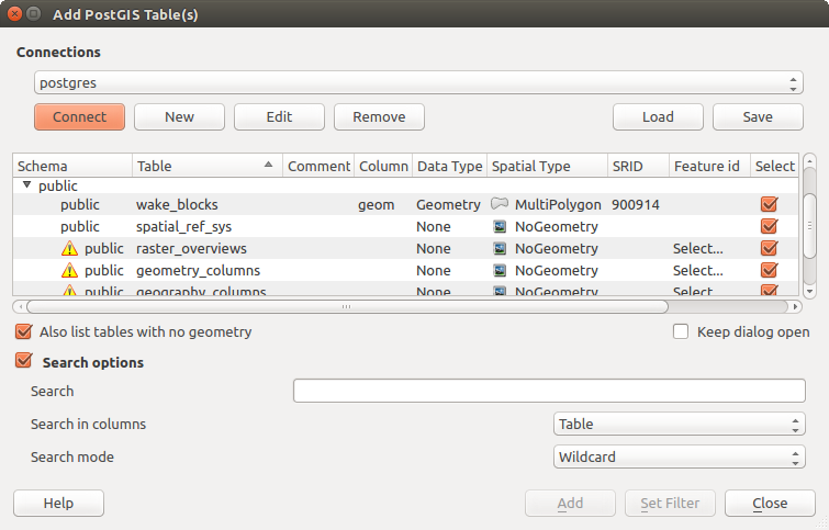
Fig. 11.16 Add PostgreSQL Table(s) Dialog
Dica
Use the Browser Panel to speed up loading of database table(s)
A adição de tabelas de BD do Gerenciador de Fonte de Dados às vezes pode ser demorado, pois o QGIS busca estatísticas e propriedades (por exemplo, tipo e campo de geometria, SRC, número de recursos) para cada tabela com antecedência. Para evitar isso, uma vez que the connection is set, é melhor usar o Browser Panel ou o DB Manager para arrastar e soltar as tabelas do banco de dados na tela do mapa.
11.1.4. The Layer Metadata Search Panel
By default, QGIS can retrieve layers metadata from the connections or data providers that allow metadata storage (more details on saving metadata to the database). The Metadata search panel allows to browse the layers by their metadata and add them to the project (either with a double-click or the Add button). The list can be filtered:
by text, watching a set of metadata properties (identifier, title, abstract)
by spatial extent, using the current project extent or the map canvas extent
by the layer (geometry) type
Nota
The sources of metadata are implemented through a layer metadata provider system that can be extended by plugins.
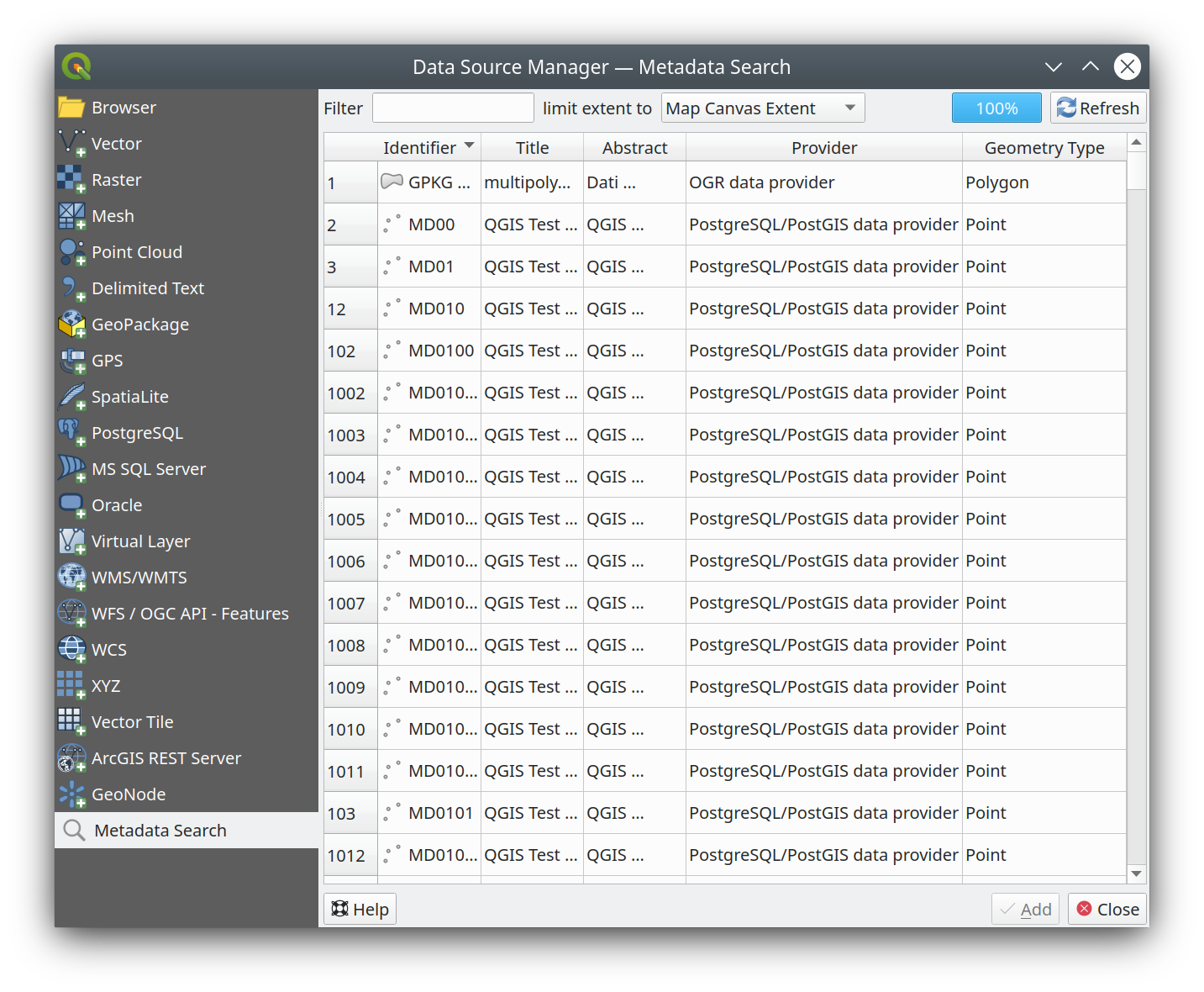
Fig. 11.17 Layer Metadata Search Panel
11.1.5. Formatos personalizados QGIS
O QGIS propõe dois formatos personalizados:
Temporary Scratch Layer: a memory layer that is bound to the project (see Creating a new Temporary Scratch Layer for more information)
Virtual Layers: a layer resulting from a query on other layer(s) (see Criando camadas virtuais for more information)
11.1.6. QLR - QGIS Layer Definition File
Layer definitions can be saved as a
Layer Definition File (QLR -
.qlr) using
in the layer
context menu.
The QLR format makes it possible to share “complete” QGIS layers with other QGIS users. QLR files contain links to the data sources and all the QGIS style information necessary to style the layer.
QLR files are shown in the Browser Panel and can be used to add layers (with their saved styles) to the Layers Panel. You can also drag and drop QLR files from the system file manager into the map canvas.
Available actions for QLR files in the Browser Panel are:
Adicionar camada ao projeto
Propriedades da Camada…
11.1.7. Conectando-se a serviços da web
With QGIS you can get access to different types of OGC web services (WM(T)S, WFS(-T), WCS, CSW, …). Thanks to QGIS Server, you can also publish such services. Guia/Manual do Servidor QGIS contains descriptions of these capabilities.
11.1.7.1. Using Vector Tiles services
Vector Tile services can be added via the  Vector
Tiles tab of the Data Source Manager dialog or the contextual menu
of the Vector Tiles entry in the Browser panel.
Services can be either a New Generic Connection… or a
New ArcGIS Vector Tile Service Connection….
Vector
Tiles tab of the Data Source Manager dialog or the contextual menu
of the Vector Tiles entry in the Browser panel.
Services can be either a New Generic Connection… or a
New ArcGIS Vector Tile Service Connection….
Você cria um serviço, adicionando:
um Nome
a Style URL: a URL to a MapBox GL JSON style configuration. If provided, then that style will be applied whenever the layers from the connection are added to QGIS. In the case of Arcgis vector tile service connections, the URL overrides the default style configuration specified in the server configuration.
You can load vector tiles directly from a Style URL. The data source is automatically parsed from the style, and URLs with multiple sources are supported. That makes Source URL optional.
the Source URL: of the type
http://example.com/{z}/{x}/{y}.pbffor generic services andhttp://example.com/arcgis/rest/services/Layer/VectorTileServerfor ArcGIS based services. The service must provide tiles in.pbfformat.the
Min. Zoom Level and the Max. Zoom Level.
Vector Tiles have a pyramid structure. By using these options you have the
opportunity to individually generate layers from the tile pyramid.
These layers will then be used to render the Vector Tile in QGIS.For Mercator projection (used by OpenStreetMap Vector Tiles) Zoom Level 0 represents the whole world at a scale of 1:500.000.000. Zoom Level 14 represents the scale 1:35.000.
the authentication configuration if necessary
a Referer
Fig. 11.18 shows the dialog with the Vector Tiles service configuration.

Fig. 11.18 Vector Tiles - Service configuration
Configurations can be saved to .XML file (Save Connections)
through the Vector Tiles entry in Data Source Manager
dialog or its context menu in the Browser panel.
Likewise, they can be added from a file (Load Connections).
Once a connection to a vector tile service is set, it’s possible to:
Edit the vector tile connection settings
Remover a conexão
From the Browser panel, right-click over the entry and you can also:
Add layer to project: a double-click also adds the layer
View the Layer Properties… and get access to metadata and a preview of the data provided by the service. More settings are available when the layer has been loaded into the project.
11.1.7.2. Using XYZ Tile services
XYZ Tile services can be added via the  XYZ tab
of the Data Source Manager dialog or the contextual menu of the
XYZ Tiles entry in the Browser panel.
By default, QGIS provides some default and ready-to-use XYZ Tiles services:
XYZ tab
of the Data Source Manager dialog or the contextual menu of the
XYZ Tiles entry in the Browser panel.
By default, QGIS provides some default and ready-to-use XYZ Tiles services:
- Mapzen Global Terrain, allowing an immediate
access to global DEM source for the projects.
More details and resources at https://registry.opendata.aws/terrain-tiles/
- OpenStreetMap to access the world 2D map.
Fig. 11.19 shows the dialog with the OpenStreetMap
XYZ Tile service configuration.
To add a new service, press New (respectively New Connection from the Browser panel) and provide:
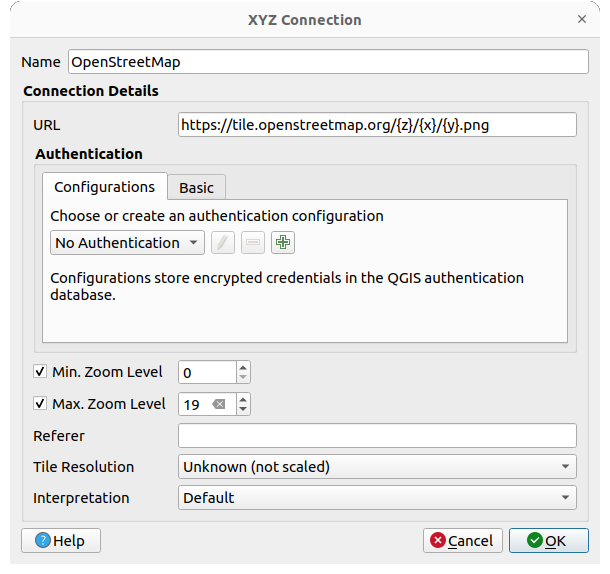
Fig. 11.19 XYZ Tiles - OpenStreetMap configuration
um Nome
the URL, you can add
http://example.com/{z}/{x}/{y}.pngorfile:///local_path/{z}/{x}/{y}.pngthe authentication configuration if necessary
the Min. Zoom level and Max. Zoom level
a Referer
the Tile Resolution: possible values are Unknown (not scaled), Standard (256x256 / 96DPI) and High (512x512 / 192DPI)
Interpretation: converts WMTS/XYZ raster datasets to a raster layer of single band float type following a predefined encoding scheme. Supported schemes are Default (no conversion is done), MapTiler Terrain RGB and Terrarium Terrain RGB. The selected converter will translate the RGB source values to float values for each pixel. Once loaded, the layer will be presented as a single band floating point raster layer, ready for styling using QGIS usual raster renderers.
Press OK to establish the connection. It will then be possible to:
Add the new layer to the project; it is loaded with the name given in the settings.
Edit the XYZ connection settings
Remover a conexão
From the Browser panel, right-click over the entry and you can also:
Add layer to project: a double-click also adds the layer
View the Layer Properties… and get access to metadata and a preview of the data provided by the service. More settings are available when the layer has been loaded into the project.
Configurations can be saved to .XML file (Save Connections)
through the XYZ entry in Data Source Manager dialog
or its contextual menu in the Browser panel.
Likewise, they can be added from a file (Load Connections).
The XML file for OpenStreetMap looks like this:
<!DOCTYPE connections>
<qgsXYZTilesConnections version="1.0">
<xyztiles url="https://tile.openstreetmap.org/{z}/{x}/{y}.png"
zmin="0" zmax="19" tilePixelRatio="0" password="" name="OpenStreetMap"
username="" authcfg="" referer=""/>
</qgsXYZTilesConnections>
Dica
Loading XYZ tiles without creating a connection
It is also possible to add XYZ tiles to a project without necessarily storing
its connection settings in you user profile (e.g. for a dataset you may need once).
In the tab, edit any properties
in the Connection Details group.
The Name field above should turn into Custom.
Press Add to load the layer in the project.
It will be named by default XYZ Layer.
Examples of XYZ Tile services:
OpenStreetMap Monochrome: URL:
http://tiles.wmflabs.org/bw-mapnik/{z}/{x}/{y}.png, Min. Zoom Level: 0, Max. Zoom Level: 19.Google Maps: URL:
https://mt1.google.com/vt/lyrs=m&x={x}&y={y}&z={z}, Min. Zoom Level: 0, Max. Zoom Level: 19.Temperatura do Mapa Meteorológico Aberto: URL:
http://tile.openweathermap.org/map/temp_new/{z}/{x}/{y}.png?appid={api_key}Nível Mín. de Zoom: 0, :guilabel: Nível Máx. de Zoom`: 19.
11.1.7.3. Using ArcGIS REST Servers
An ArcGIS REST Server can host many different types of web services
(feature service, map service, image service, …).
ArcGIS REST Servers can be added via the
 ArcGIS REST Server tab of the
Data Source Manager dialog or the contextual menu of the
ArcGIS REST Servers entry in the Browser panel:
ArcGIS REST Server tab of the
Data Source Manager dialog or the contextual menu of the
ArcGIS REST Servers entry in the Browser panel:
Press New (respectively New Connection) and provide:
a Name: A name for the connection.
the URL: Main address of the ArcGIS REST Server.
a Prefix: Used to specify the proxy prefix in the URL, which is necessary for some ArcGIS servers that use web proxy prefixes.
a Community endpoint URL: Endpoint URL for ArcGIS Online or Portal for ArcGIS, used to access content groups.
a Content endpoint URL: Endpoint URL for the content service. This is used to access items in ArcGIS Online or Portal for ArcGIS.
the authentication credentials if necessary.
a Referer: The referer URL to be sent in the HTTP headers when making requests to the server. This may be required by some servers for authentication purposes.
Nota
ArcGIS Feature Service connections which have their corresponding Portal endpoint URLS set can be explored by content groups in the browser panel.
Se uma conexão tiver os terminais do Portal definidos, expandir a conexão no navegador mostrará uma pasta “Grupos” e “Serviços”, em vez da lista completa de serviços normalmente exibida. Expandir a pasta de grupos mostrará uma lista de todos os grupos de conteúdo dos quais o usuário é membro, cada um dos quais pode ser expandido para mostrar os itens de serviço pertencentes a esse grupo.
Then press OK to validate the configuration settings. These configurations can be saved to
.XMLfile (Save). Likewise, they can be added from a file (Load).Once a connection to an ArcGIS REST Server is set, it is possible to:
Edit the ArcGIS REST Server connection settings
Remover a conexão
Refresh the connection
Press Connect to request the server and display its contents. They are organized in a tree structure whose nodes depend on the connection’s endpoint.

Fig. 11.20 Data Source Manager - ArcGIS REST Server
Expand the tree to find and select the layers of interest. Their Coordinate Reference System is displayed at the bottom of the dialog.
For raster-based layers, you can select the Image encoding to use among a number of image formats advertised by the target service ( e.g.,
PNG,JPG,GIF,SVG,SVGZ, … ).To add the selected layers to the map canvas, press Add button.
Because layers can sometimes load and render slowly on the client side, applying a filter to restrict the features retrieved from the service can significantly improve performance, since only the filtered features are requested from the server. This can be done by:
checking
Only request features overlapping the current view extentfor vector layers (feature service), pressing Add with filter to apply attribute-based filters to the layer with O Construtor de string de expressão functions.
In the Browser panel, right-click the ArcGIS REST Server layer and select Add Filtered Layer to Project will also open the builder dialog.
Most of the above tools to connect and access layers on an ArcGIS REST Server are also available from the Browser panel, within the contextual menu of the target node item. Depending on the node, you can also:
View Service Info which will open the default web browser and display information on the requested service.
View the Layer Properties… and get access to the metadata and a preview of the data provided by the service. More settings are available when the layer has been loaded into the project.
11.1.7.4. Using 3D tiled scene services
QGIS supports multiple formats of 3D tiled datasets, grouped together as “tiled scenes”. These include Cesium 3D Tiles and Quantized Mesh tiles.
To load a tiled scene dataset into QGIS, use the  Scene tab in the Data Source Manager dialog.
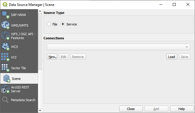
Fig. 11.21 Data Source Manager - Scene
Create a connection by clicking on New. You can add a New Cesium 3D Tiles Connection or a New Quantized Mesh Connection.
Choose a Name and set the URL to the URL of a layer description JSON file.
The URL may be remote (e.g. http://example.com/tileset.json) or local (e.g.
file:///path/to/tiles/tileset.json).
The authentication configuration if necessary.
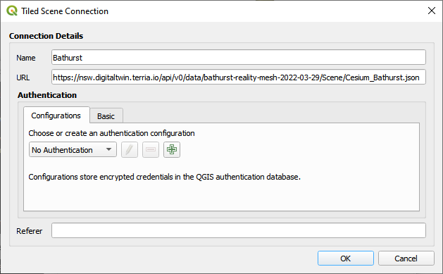
Fig. 11.22 Tiled Scene Connection
You can also add the service from Browser Panel.
After creating new connection you are able to Add the new layer to your map.
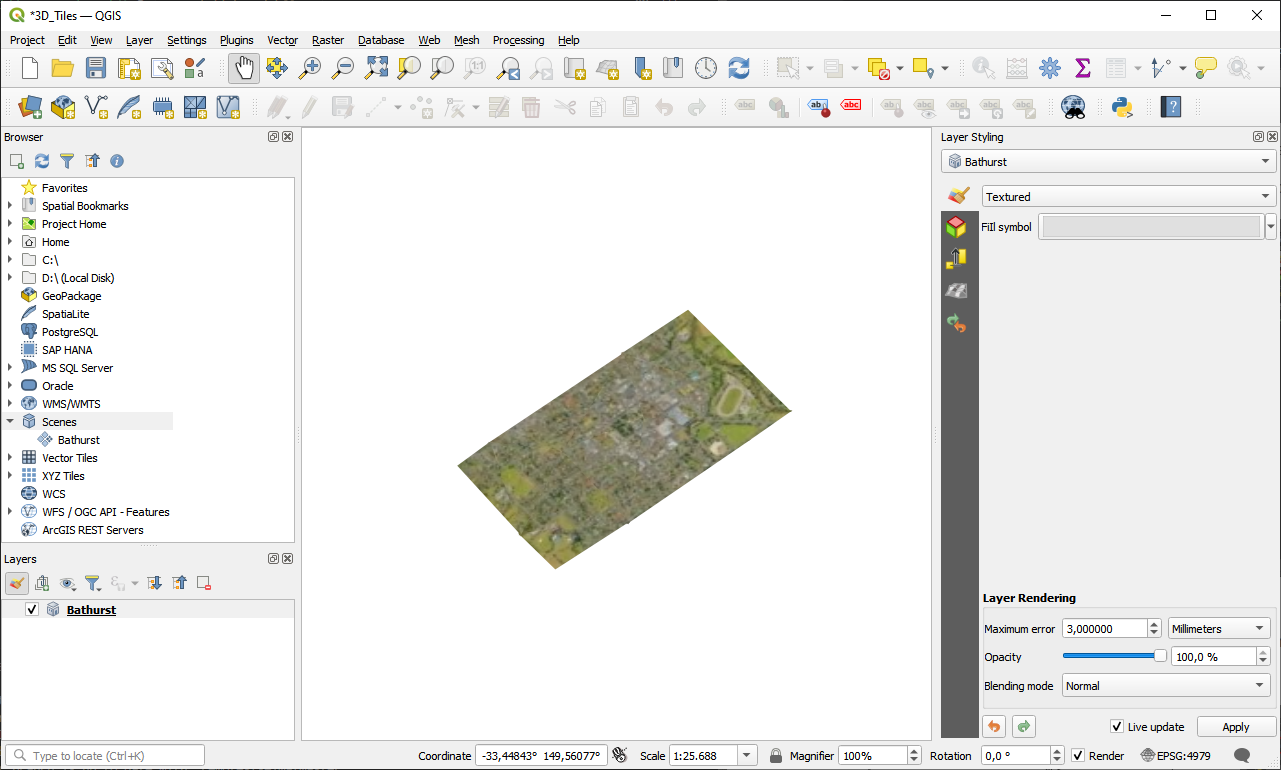
Fig. 11.23 3D Tiles Layer - Textured

Fig. 11.24 Quantized Mesh layer
11.1.7.5. Using Cloud Connections
QGIS supports connections to cloud services like Alibaba Cloud OSS, Amazon S3, Google Cloud Storage,
Microsoft Azure Blob Storage, Microsoft Azure Data Lake Storage, and OpenStack Swift Object Storage.
You can load vector and raster data from these services into QGIS.
Set up a new  Cloud connection in the Browser panel by right-clicking
on the Cloud entry and selecting New Connection. You will see a drop-down list of
available cloud services.
Select the service you want to connect to and fill in the required fields:
Cloud connection in the Browser panel by right-clicking
on the Cloud entry and selecting New Connection. You will see a drop-down list of
available cloud services.
Select the service you want to connect to and fill in the required fields:

Fig. 11.25 Cloud Connection Dialog
Name: A name for the connection.
Bucket or Container: The name of the bucket or container in the cloud service.
Object Key (optional): The key of the object in the bucket or container.
Credentials: The credentials to access the cloud service.
You can also choose to Save Connection to an XML file or Load Connection from an XML file.