7.3. Lesson: Análisis del Terreno

Ciertos tipos de ráster te permiten obtener una visión más clara del terreno que representan. Los Modelos de Digital de Elevaciones (MDEs) son particularmente útiles para ello. En esta lección utilizaras herramientas de análisis de terrenos para obtener más información sobre el área de estudio para la propuesta de desarrollo residencial anterior.

El objetivo de esta lección: Utilizar herramientas de análisis del terreno para obtener más información sobre el terreno.

7.3.1. Follow Along: Cálculo del Relieve Sombreado

We are going to use the same DEM layer as in the previous lesson. If you are starting this chapter from scratch, use the Browser panel and load the raster/SRTM/srtm_41_19.tif.

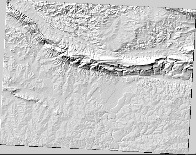
The DEM layer shows you the elevation of the terrain, but it can sometimes seem a little abstract. It contains all the 3D information about the terrain that you need, but it doesn’t look like a 3D object. To get a better impression of the terrain, it is possible to calculate a hillshade, which is a raster that maps the terrain using light and shadow to create a 3D-looking image.

We are going to use algorithms in the Raster ► Raster terrain analysis menu.

1. Click on the Hillshade menu

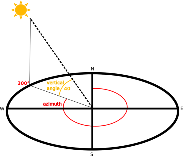
2. The algorithm allows you to specify the position of the light source: Azimuth has values from 0 (North) through 90 (East), 180 (South) and 270 (West), while the Vertical angle sets how high the light source is (0 to 90 degrees).

3. Usaremos os seguintes valores:

   • guilabel:Fator Z em 1,0`

   • Azimuth (horizontal angle) at 300.0°

   • Vertical angle at 40.0°

   

4. Save the file in a new folder exercise_data/raster_analysis/ with the name hillshade

5. Finalmente clique em Executar.

Ahora tendrás una capa nueva llamada relieve_sombreado que tiene este aspecto:

Se ve bien en 3D, pero ¿podemos mejorarla? En sí mismo, el sombreado del relieve parece un molde de yeso. ¿No podríamos utilizarlo con nuestros otros ráster más coloridos de alguna manera? Por supuesto que podemos, utilizando el sombreado del relieve como una capa sobrepuesta.

7.3.2. Follow Along: Utilizando un Sombreado del Relieve como Capa Sobrepuesta

Un sombreado del relieve puede proporcionar información muy útil sobre la luz solar en un momento dado del día. Pero también puede ser utilizado para fines estéticos, para que el mapa tenga mejor aspecto. La clave en este caso está en que el sombreado del relieve sea defina como mayormente transparente.

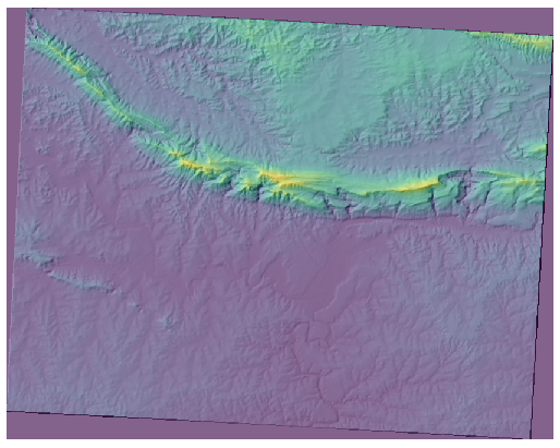
1. Change the symbology of the original srtm_41_19 layer to use the Pseudocolor scheme as in the previous exercise

2. Hide all the layers except the srtm_41_19 and hillshade layers

3. Click and drag the srtm_41_19 to be beneath the hillshade layer in the Layers panel

4. Set the hillshade layer to be transparent by clicking on the Transparency tab in the layer properties

5. Set the Global opacity to 50%.

   Você obterá um resultado como este:

   

6. Switch the hillshade layer off and back on in the Layers panel to see the difference it makes.

Utilizando el sombreado del relieve de esta forma, es posible enaltecer la topografía del paisaje. Si el efecto no parece ser suficiente para ti, puedes cambiar la transparencia de la capa relieve_sombreado, pero por supuesto, cuanto más brillante se vuelva el sombreado del relieve, peor se verán los colores bajo él. Necesitarás encontrar un balance que funcione.

Lembre-se de salvar o projeto quando terminar.

7.3.3. Follow Along: Finding the best areas

Think back to the estate agent problem, which we last addressed in the Vector Analysis lesson. Let us imagine that the buyers now wish to purchase a building and build a smaller cottage on the property. In the Southern Hemisphere, we know that an ideal plot for development needs to have areas on it that:

• estão voltados para o norte

• com inclinação inferior a 5 graus

• Mas se a inclinação for inferior a 2 graus, o aspecto não importa.

Vamos encontrar as melhores áreas para eles.

7.3.4. Follow Along: Calculo de la Pendiente

Inclinação informa sobre a inclinação do terreno. Se, por exemplo, você quiser construir casas no terreno, precisará de um terreno relativamente plano.

To calculate the slope, you need to use the Slope algorithm of the Processing ► Raster terrain analysis.

1. Abrir o algoritmo

2. Choose srtm_41_19 as the Elevation layer

3. Keep the Z factor at 1.0

4. Save the output as a file with the name slope in the same folder as the hillshade

5. Clique em Executar

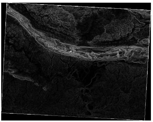
Now you’ll see the slope of the terrain, each pixel holding the corresponding slope value. Black pixels show flat terrain and white pixels, steep terrain:

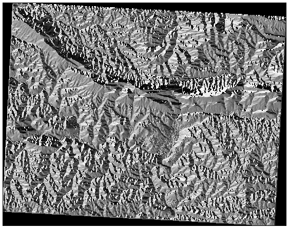
7.3.5. Try Yourself Calculating the aspect

Aspect is the compass direction that the slope of the terrain faces. An aspect of 0 means that the slope is North-facing, 90 East-facing, 180 South-facing, and 270 West-facing.

Como esse estudo está ocorrendo no Hemisfério Sul, as casas devem idealmente ser construídas em uma encosta voltada para o norte, para que possam permanecer à luz do sol.

Use the Aspect algorithm of the Processing ► Raster terrain analysis to get the aspect layer saved along with the slope.

Resposta

Set your Aspect dialog up like this:

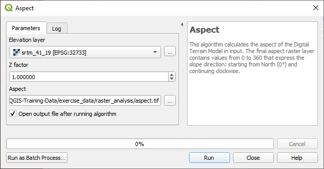
Seu resultado:

7.3.6. Follow Along: Finding the north-facing aspect

Now, you have rasters showing you the slope as well as the aspect, but you have no way of knowing where ideal conditions are satisfied at once. How could this analysis be done?

La respuesta está en la Calculadora ráster.

O QGIS tem diferentes calculadoras raster disponíveis:

• Raster ► Raster Calculator

• Em processo:

  • Raster Analysis ► Raster calculator

  • GDAL ► Raster miscellaneous ► Raster calculator

  • SAGA ► Raster calculus ► Raster calculator

Each tool is leading to the same results, but the syntax may be slightly different and the availability of operators may vary.

We will use Raster Analysis ► Raster calculator in the Processing Toolbox

1. Open the tool by double clicking on it.

   • The upper left part of the dialog lists all the loaded raster layers as name@N, where name is the name of the layer and N is the band.

   • In the upper right part you will see a lot of different operators. Stop for a moment to think that a raster is an image. You should see it as a 2D matrix filled with numbers.

2. North is at 0 (zero) degrees, so for the terrain to face north, its aspect needs to be greater than 270 degrees or less than 90 degrees. Therefore the formula is:

   aspect@1 <= 90 OR aspect@1 >= 270
   

3. Now you have to set up the raster details, like the cell size, extent and CRS. This can be done manually or it can be automatically set by choosing a Reference layer. Choose this last option by clicking on the … button next to the Reference layer(s) parameter.

4. In the dialog, choose the aspect layer, because we want to obtain a layer with the same resolution.

5. Save the layer as aspect_north.

   The dialog should look like:

   

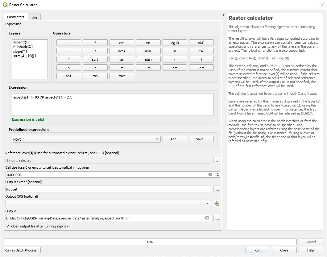
6. Finalmente clique em Executar.

Tu resultado será este:

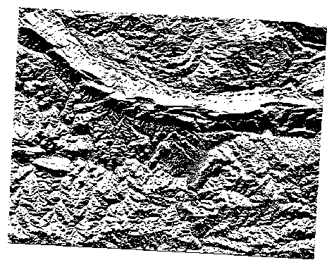
The output values are 0 or 1. What does it mean? For each pixel in the raster, the formula we wrote returns whether it matches the conditions or not. Therefore the final result will be False (0) and True (1).

7.3.7. Try Yourself More criteria

Now that you have done the aspect, create two new layers from the DEM.

• The first shall identify areas where the slope is less than or equal to 2 degrees

• The second is similar, but the slope should be less than or equal to 5 degrees.

• Save them under exercise_data/raster_analysis as slope_lte2.tif and slope_lte5.tif.

Resposta

• Set your Raster calculator dialog up with:

• the following expression: slope@1 <= 2

• the slope layer as the Reference layer(s)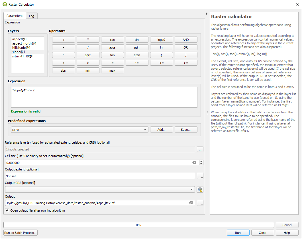

  

• For the 5 degree version, replace the 2 in the expression and file name with 5.

Seus resultados:

• 2 graus:

  

• 5 graus:

  

7.3.8. Follow Along: Combinando Resultados de Análisis Ráster

Agora você gerou três camadas raster do MDE:

• aspect_north: terrain facing north

• slope_lte2: slope equal to or below 2 degrees

• slope_lte5: slope equal to or below 5 degrees

Where the condition is met, the pixel value is 1. Elsewhere, it is 0. Therefore, if you multiply these rasters, the pixels that have a value of 1 for all of them will get a value of 1 (the rest will get 0).

As condições a cumprir são:

• at or below 5 degrees of slope, the terrain must face north

• at or below 2 degrees of slope, the direction that the terrain faces does not matter.

Therefore, you need to find areas where the slope is at or below five degrees AND the terrain is facing north, OR the slope is at or below 2 degrees. Such terrain would be suitable for development.

Para calcular las áreas que cumplen esos criterios:

1. Open the Raster calculator again

2. Use this expression in Expression:

   ( aspect_north@1 = 1 AND slope_lte5@1 = 1 ) OR slope_lte2@1 = 1
   

3. Set the Reference layer(s) parameter to aspect_north (it does not matter if you choose another - they have all been calculated from srtm_41_19)

4. Save the output under exercise_data/raster_analysis/ as all_conditions.tif

5. Clique em :guilabel:` Executar `

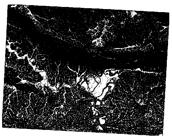
O resultado:

Dica

As etapas anteriores poderiam ter sido simplificadas usando o seguinte comando:

((aspect@1 <= 90 OR  aspect@1 >= 270) AND slope@1 <= 5) OR slope@1 <= 2

7.3.9. Follow Along: Simplificando el Ráster

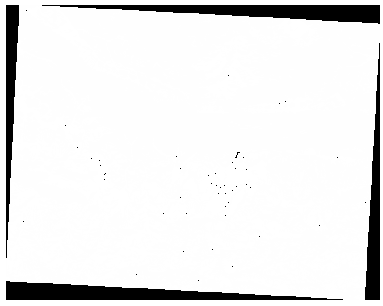
As you can see from the image above, the combined analysis has left us with many, very small areas where the conditions are met (in white). But these aren’t really useful for our analysis, since they are too small to build anything on. Let us get rid of all these tiny unusable areas.

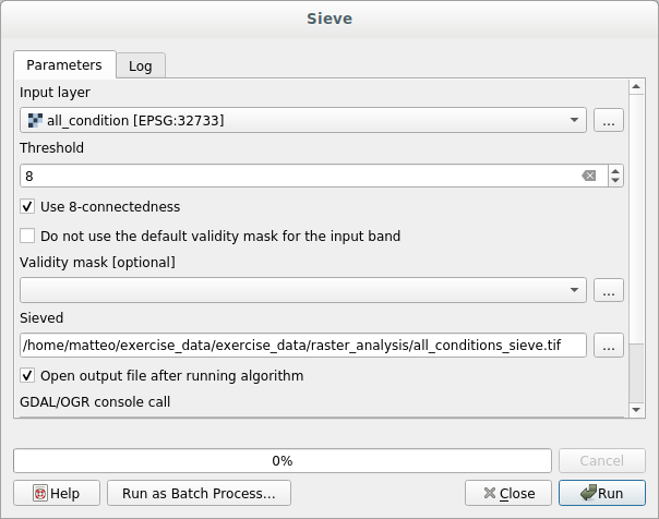
1. Open the Sieve tool (GDAL ► Raster Analysis in the Processing Toolbox)

2. Set the Input file to all_conditions, and the Sieved to all_conditions_sieve.tif (under exercise_data/raster_analysis/).

3. Set the Threshold to 8 (minimum eight contiguous pixels), and check Use 8-connectedness.

   

   Uma vez concluído o processamento, a nova camada será carregada.

   

   What is going on? The answer lies in the new raster file’s metadata.

4. View the metadata under the Information tab of the Layer Properties dialog. Look the STATISTICS_MINIMUM value: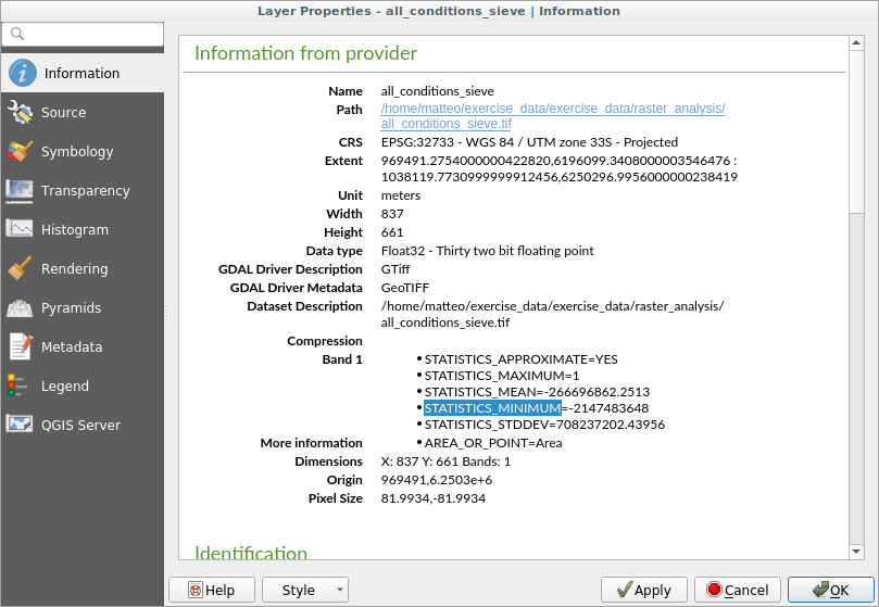

   

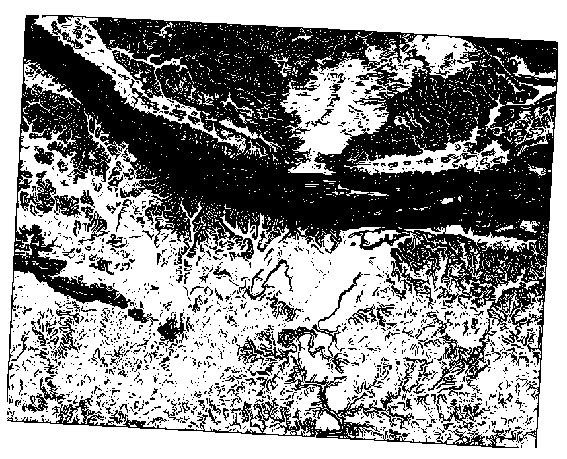
   This raster, like the one it is derived from, should only feature the values 1 and 0, but it has also a very large negative number. Investigation of the data shows that this number acts as a null value. Since we are only after areas that weren’t filtered out, let us set these null values to zero.

5. Abra a :guilabel:’Calculadora Raster’, e construa esta expressão:

   (all_conditions_sieve@1 <= 0) = 0
   

   Isso manterá todos os valores não negativos e definirá os números negativos como zero, deixando todas as áreas com valor 1 intactas.

6. Save the output under exercise_data/raster_analysis/ as all_conditions_simple.tif.

Tu resultado tiene este aspecto:

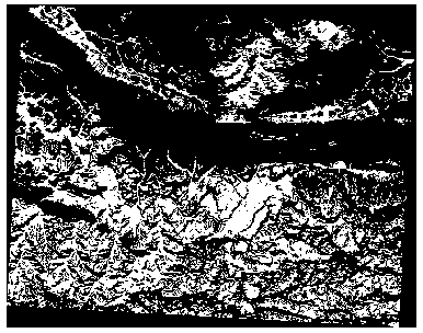
Eso era lo que se esperaba: una versión simplificada de los resultados anteriores. Recuerda que si los resultados que obtienes de una herramienta no son los que esperabas, comprobando los metadatos (y atributos vectoriales, si es aplicable) puede ser esencial para solucionar el problema.

7.3.10. Follow Along: Reclassifying the Raster

Usamos a Calculadora Raster para fazer cálculos em camadas raster. Existe outra ferramenta poderosa que podemos usar para extrair informações das camadas existentes.

Back to the aspect layer. We know now that it has numerical values within a range from 0 through 360. What we want to do is to reclassify this layer to other discrete values (from 1 to 4), depending on the aspect:

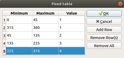
• 1 = Norte (de 0 a 45 e de 315 a 360);

• 2 = Leste (de 45 a 135)

• 3 = Sul (de 135 a 225)

• 4 = Oeste (de 225 a 315)

Essa operação pode ser realizada com a calculadora raster, mas a fórmula ficaria muito grande.

The alternative tool is the Reclassify by table tool in Raster analysis in the Processing Toolbox.

1. Abra a ferramenta

2. Choose aspect as the Input raster layer

3. Click on the … of Reclassification table. A table-like dialog will pop up, where you can choose the minimum, maximum and new values for each class.

4. Clique no botão Adicionar linha e adicione 5 linhas. Preencha cada linha como a seguinte figura e clique em OK:

   

   The method used by the algorithm to treat the threshold values of each class is defined by the Range boundaries.

5. Save the layer as reclassified.tif in the exercise_data/raster_analysis/ folder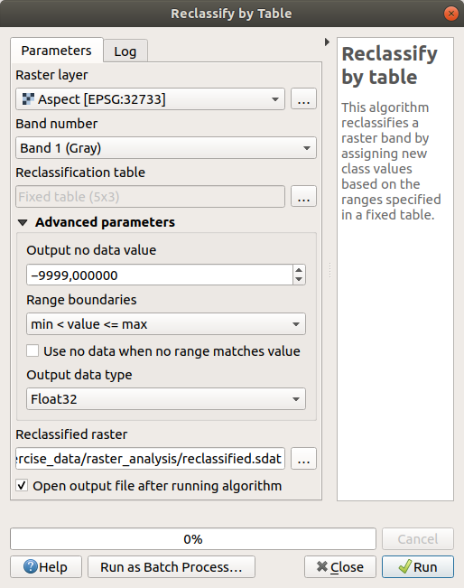

   

6. Clique em Executar

If you compare the native aspect layer with the reclassified one, there are not big differences. But by looking at the legend, you can see that the values go from 1 to 4.

Vamos dar um estilo melhor a esta camada.

1. Open the Layer Styling panel

2. Choose Paletted/Unique values, instead of Singleband gray

3. Click on the Classify button to automatically fetch the values and assign them random colors:

   

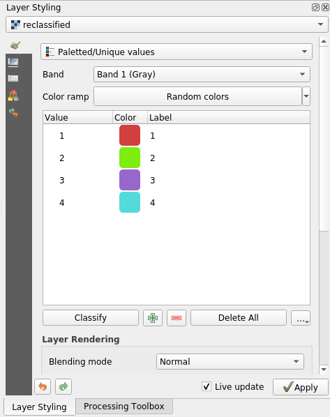
A saída deve ficar assim (você pode ter cores diferentes, pois foram geradas aleatoriamente):

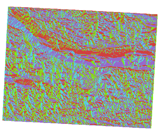
With this reclassification and the paletted style applied to the layer, you can immediately differentiate the aspect areas.

7.3.11. Follow Along: Querying the raster

Unlike vector layers, raster layers don’t have an attribute table. Each pixel contains one or more numerical values (singleband or multiband rasters).

All the raster layers we used in this exercise consist of just one band. Depending on the layer, pixel values may represent elevation, aspect or slope values.

How can we query the raster layer to get the value of a pixel? We can use the ^{Identify Features} button!

1. Selecione a ferramenta na barra de ferramentas Atributos.

2. Click on a random location of the srtm_41_19 layer. Identify Results will appear with the value of the band at the clicked location:

   

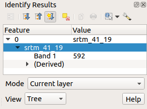
3. You can change the output of the Identify Results panel from the current tree mode to a table one by selecting Table in the View menu at the bottom of the panel: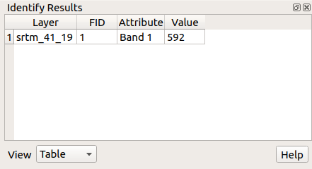

   

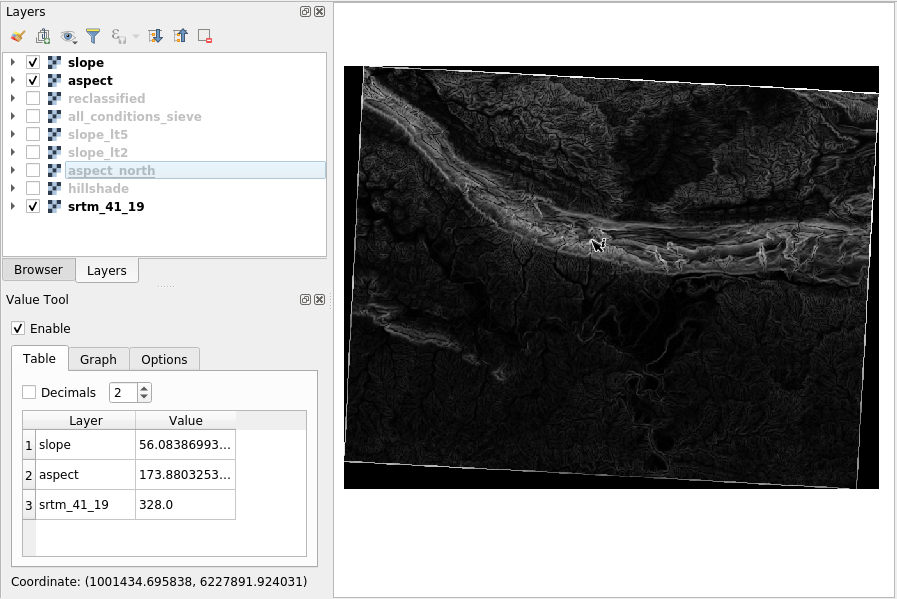
Clicking each pixel to get the value of the raster could become annoying after a while. We can use the Value Tool plugin to solve this problem.

1. Vá para Complementos ► Gerenciar/Instalar Complementos…

2. In the All tab, type value t in the search box

3. Select the Value Tool plugin, press Install Plugin and then Close the dialog.

   

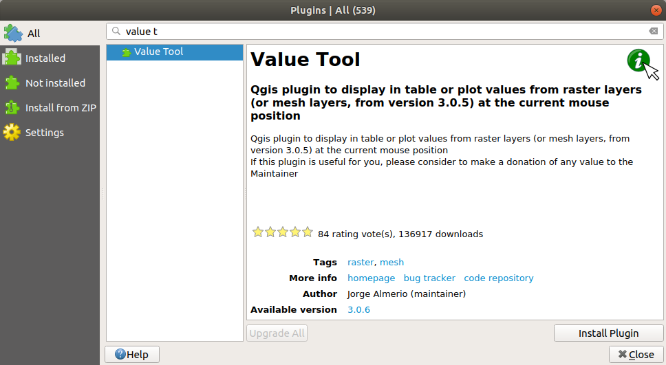
   The new Value Tool panel will appear.

   Dica

   If you close the panel you can reopen it by enabling it in the View ► Panels ► Value Tool or by clicking on the icon in the toolbar.

4. To use the plugin just check the Enable checkbox and be sure that the srtm_41_19 layer is active (checked) in the Layers panel.

5. Mova o cursor sobre o mapa para ver o valor dos pixels.

   

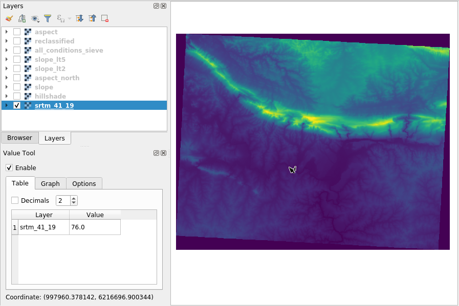
6. But there is more. The Value Tool plugin allows you to query all the active raster layers in the Layers panel. Set the aspect and slope layers active again and hover the mouse on the map:

   

7.3.12. In Conclusion

You’ve seen how to derive all kinds of analysis products from a DEM. These include hillshade, slope and aspect calculations. You’ve also seen how to use the raster calculator to further analyze and combine these results. Finally you learned how to reclassify a layer and how to query the results.

7.3.13. What’s Next?

Ahora tienes dos análisis: el análisis vectorial que te muestra las parcelas potencialmente adecuadas, y el análisis ráster que te muestra el terreno potencialmente adecuado. ¿Cómo se pueden combinar para llegar a un resultado final para este problema? Ese es el tema de la siguiente lección, empezando en el módulo siguiente.