14.5. Lesson: Design da Amostragem Sistemática
Já digitalizou um conjunto de polígonos que representam povoamentos florestais, mas ainda não tem informações sobre a floresta. Para esse efeito, pode projetar uma pesquisa para o inventário da área de floresta e, em seguida, estimar os seus parâmetros. Nesta lição, vai criar um conjunto de pontos de amostragem sistemática.
Quando começamos a planear um inventário florestal é importante definir claramente os objetivos, os tipos de parcelas que vão ser utilizados, e os dados que serão recolhidos para atingir os objectivos. Para cada caso individual, irá depender do tipo de gestão da floresta proposta; e deve ser cuidadosamente planeado por alguém com conhecimento na área florestal. Nesta lição, vai implementar um inventário teórico baseado numa amostragem sistemática de parcelas.
**O objetivo desta lição:**Criar um esquema de parcelas de amostragem sistemática com o intuito de fazer o levantamento da área florestal.
14.5.1. Inventariar a Floresta
Existem diversos métodos de inventariar a floresta, cada um com diferentes condições e propósitos. Por exemplo, de uma forma muito precisa para inventariar uma floresta (se considerar apenas espécies de árvores) seria visitar a floresta e fazer uma lista de todas as árvores e as suas características. Como pode imaginar este não é geralmente aplicável excepto para áreas pequenas ou situações especiais.
The most common way to find out about a forest is by sampling it, that is, taking measurements in different locations at the forest and generalizing that information to the whole forest. These measurements are often made in sample plots that are smaller forest areas that can be easily measured. The sample plots can be of any size (for ex. 50 m2, 0.5 ha) and form (for ex. circular, rectangular, variable size), and can be located in the forest in different ways (for ex. randomly, systematically, along lines). The size, form and location of the sample plots are usually decided following statistical, economical and practical considerations. If you have no forestry knowledge, you might be interested in reading this Wikipedia article.
14.5.2.  Follow Along: Implementação do design da amostragem sistemática
Para a floresta que está a trabalhar, o gestor decidiu que o design da amostragem sistemática como o mais apropriado para esta floresta decidindo que a distância entre as parcelas seria fixa, com 80 metros entre as linhas de amostragem visto que iria produzir resultados confiáveis (para este caso, + - 5% de erro médio a uma probabilidade de 68%). Como o método mais eficaz para este inventário decidiu-se que as parcelas teriam tamanho variável, para os povoamentos em crescimento e maduros, para povoamentos jovens seriam usadas parcelas de raio fixo com 4 metros de raio.
Na prática, necessita de simplesmente representar as parcelas de amostra como pontos que serão usados pelas equipas de campo posteriormente:
Open your
digitizing_2012.qgsproject from the previous lesson.Remove all the layers except for forest_stands_2012.
Save your project now as
forest_inventory.qgs
Agora necessita de criar uma grelha retangular de pontos separados por 80 metros um do outro:
Open
 Regular points.
Press the drop-down button next to the Input extent field and from the Calculate from Layer menu, select forest_stands_2012.
In the Point spacing/count settings, enter
80meters.Check the Use point spacing box to indicate that the value represents the distance between the points.
Under Regular points, save the output as
systematic_plots.shpin theforestry\sampling\folder.Check Open output file after running algorithm.
Press Run.
Nota
The suggested Regular points creates the systematic points starting in the upper-left corner of the extent of the selected polygon layer. If you want to add some randomness to this regular points, you could use a randomly calculated number between 0 and 80 (80 is the distance between our points), and then write it as the Initial inset from corner (LH side) parameter in the tool’s dialog.
Percebe que a ferramenta usa toda a extensão da sua camada de povoamentos para gerar uma grelha retangular de pontos. Mas interessa-nos apenas esses pontos que estão, na verdade, dentro da sua área de floresta (veja as imagens abaixo):
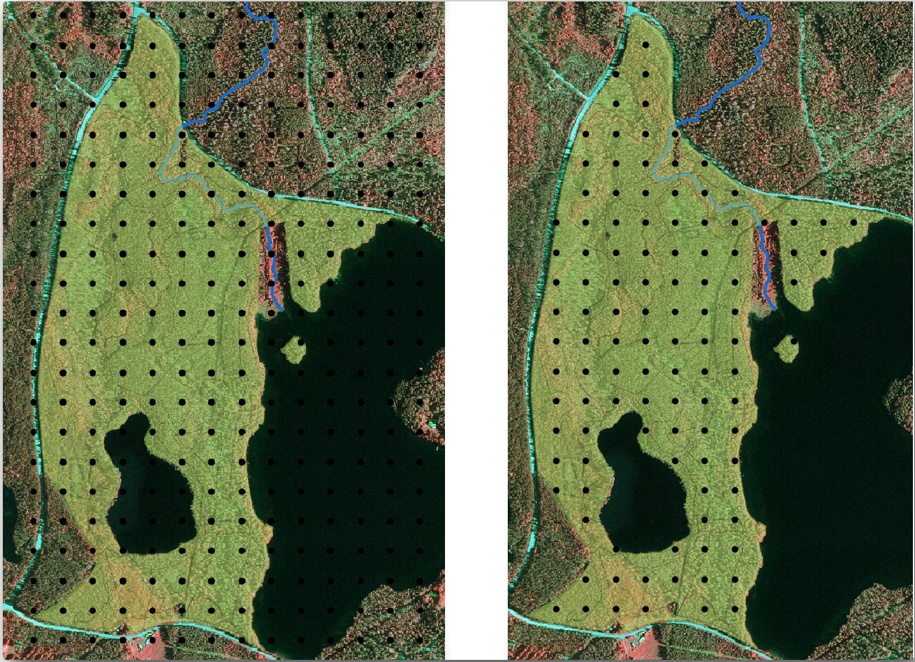
From the Processing toolbox, open
 .
.Select systematic_plots as the Input layer.
Set forest_stands_2012 as the Mask layer.
Save the Clipped (mask) result as
systematic_plots_clip.shpin theforestry\sampling\folder.Check Open output file after running algorithm.
Press Run.
Tem agora os pontos que as equipas de campo vão usar para navegar até os locais das parcelas planeadas. Pode ainda preparar estes pontos de modo a que eles sejam mais úteis para o trabalho de campo. Pelo menos terá que adicionar nomes significativos para os pontos e exportá-los para um formato que pode ser usado no seu aparelho de GPS.
Let’s start with the naming of the sample plots. If you check the Attribute table for the plots inside the forest area, you can see that you have the default id field automatically generated by the Regular points tool. Label the points to see them in the map and consider if you could use those numbers as part of your sample plot naming:
Open the
 Labels
for the
Labels
for the systematic_plots_cliplayer.Turn the top menu into
Single Labels.For the Value entry, select the field
id.Go to the
 Buffer tab, check the
Draw text buffer and set the buffer Size to
Buffer tab, check the
Draw text buffer and set the buffer Size to 1.Click OK.
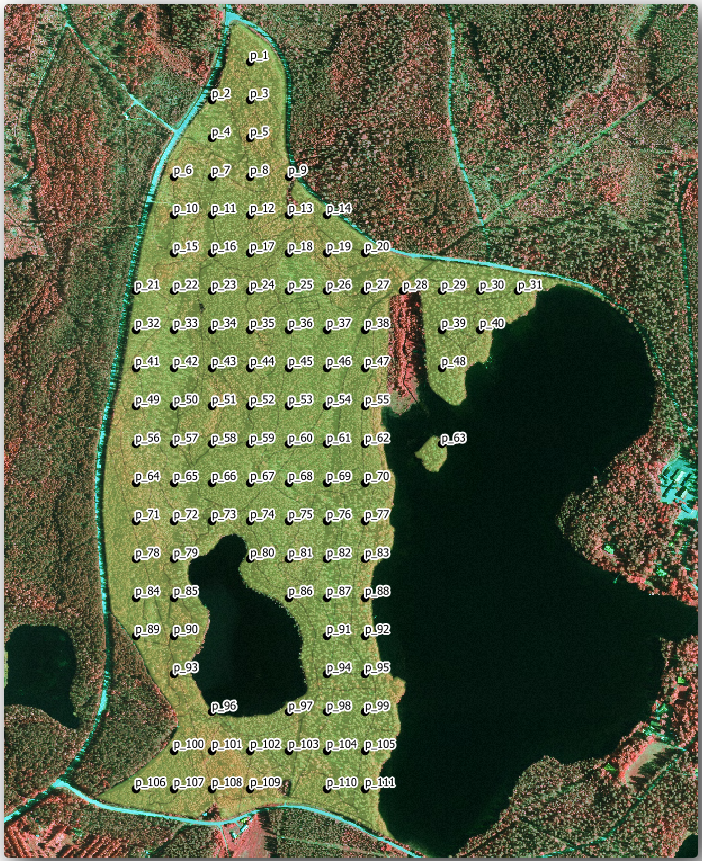
Agora olhe para os rótulos do seu mapa. Pode verificar que os pontos foram criadas e numeradas primeiro de Ocidente para o Oriente e, em seguida, do Norte para o Sul. Se olhar para a tabela de atributos de novo, vai notar que a ordem na tabela também segue esse padrão. Se pretender nomear por outras razões as parcelas de uma forma diferente, nomeando-os de uma forma Leste-Oeste / Norte-Sul segue uma ordem lógica e é uma boa opção.
Nevertheless, the number values in the id field are not so good.
It would be better if the naming would be something like p_1, p_2....
You can create a new column for the systematic_plots_clip layer:
Go to the Attribute table for
systematic_plots_clip.Enable the
 edit mode.
Open the
 Field calculator:
Check Create a new field
Enter
Plot_idas Output field nameSet the Output field type to Text (string).
In the Expression field, write, copy or construct this formula
concat('P_', @rownum ). Remember that you can also double click on the elements inside the Function list. Theconcatfunction can be found under String and@rownumis under the Variables and values group.
Click OK.
Desactive o modo de edição e guarde as alterações.
Now you have a new column with plot names that are meaningful to you. For the
systematic_plots_clip layer, change the field used for labeling to your
new Plot_id field.
14.5.3. Follow Along: Exportar a amostra de parcelas como formato GPX
The field teams will be probably using a GPS device to locate the sample plots you planned. The next step is to export the points you created to a format that your GPS can read. QGIS allows you to save your point and line vector data in GPS eXchange Format (GPX), which is an standard GPS data format that can be read by most of the specialized software. You need to be careful with selecting the CRS when you save your data:
Right-click
systematic_plots_cliplayer and select .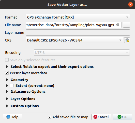
Em Formato seleccione GPS eXchange Format [GPX].
Save the output File name as
plots_wgs84.gpxin theforestry\sampling\folder.Em SRC selecionar Seleccionar SRC.
Browse for EPSG:4326 - WGS 84.
Nota
The GPX format accepts only this CRS, if you select a different one, QGIS will give no error but you will get an empty file.
Click OK.
In the dialog that opens, select only the
waypointslayer (the rest of the layers are empty).
The inventory sample plots are now in a standard format that can be managed by
most of the GPS software. The field teams can now upload the locations of the
sample plots to their devices. That would be done by using the specific devices
own software and the plots_wgs84.gpx file you just saved. Other option
would be to use the GPS Tools plugin but it would most likely
involve setting the tool to work with your specific GPS device. If you are
working with your own data and want to see how the tool works you can find out
information about it in the section Trabalhando com dados GPS in the QGIS User Manual.
Guarde o seu projecto QGIS
14.5.4. In Conclusion
Acabou de ver como poderá criar facilmente um projeto de amostragem sistemática para ser usado num inventário florestal. A criação de outros tipos de planos de amostragem envolve o uso de diferentes ferramentas dentro do QGIS, folhas de cálculo ou scripts para calcular as coordenadas das parcelas, mas a ideia geral permanece a mesma.
14.5.5. What’s Next?
Na próxima lição verá como usar os recursos do atlas no QGIS para gerar automaticamente mapas detalhados que as equipas de campo usam para navegar para as parcelas que lhes foram atribuídas.