중요
번역은 여러분이 참여할 수 있는 커뮤니티 활동입니다. 이 페이지는 현재 91.30% 번역되었습니다.
6.2. 수업: 벡터 분석
서로 다른 피처들이 공간에서 어떻게 쌍방향 작용을 하는지 밝히기 위해 벡터 데이터를 분석할 수도 있습니다. 서로 다른 분석 관련 기능들이 많이 있기 때문에, 전부를 살펴보지는 않을 것입니다. 그보다는, 질문을 상정하고 QGIS가 제공하는 도구들을 사용해서 해결하려 해볼 것입니다.
이 수업의 목표: 문제를 제시하고, 분석 도구를 써서 해결하기
6.2.1. ★☆☆ GIS 처리 과정
시작하기 전에, 문제를 해결하기 위해 사용할 수 있는 처리 과정의 간단한 개요를 알아두는 편이 유용할 것입니다. 그 개요란 다음과 같습니다:
문제를 정의
데이터 획득
문제를 분석
결과를 제시
6.2.2. ★☆☆ 문제
해결해야 할 문제를 결정하는 것으로 처리 과정을 시작합시다. 예를 들어 여러분이 부동산 업자인데 다음 기준을 가진 고객을 위해 Swellendam 에 있는 거주지를 찾고 있다고 해봅시다:
Swellendam 에 있어야 한다.
학교에서 적정한 운전 거리 (1km 정도) 안에 있어야 한다.
면적은 100평방미터 이상이어야 한다.
주요 도로에서 50미터 이상 떨어져서는 안 된다.
500미터 반경 안에 식당이 있어야 한다.
6.2.3. ★☆☆ 데이터
이 질문들에 답하려면, 다음 데이터가 필요할 겁니다:
이 지역의 거주 부지 (건물)
도시 내부 및 주면의 도로
학교와 식당의 위치
건물의 면적
이런 데이터는 오픈스트리트맵을 통해 구할 수 있으며, 지금까지 이 교재를 공부하며 사용했던 데이터셋도 사용할 수 있을 것입니다.
다른 지역의 데이터를 다운로드 받고 싶다면, 예제 데이터 준비 에서 그 방법을 읽어보십시오.
참고
오픈스트리트맵 다운로드는 일관된 데이터 항목을 가지고 있지만, 커버리지 및 세부 내용은 다를 수 있습니다. 예를 들어 여러분이 선택한 지역에 식당 정보가 없다면, 다른 지역을 선택해야 할 수도 있습니다.
6.2.4. ★☆☆ 따라해보세요: 프로젝트를 시작하고 데이터를 가져오기
먼저 작업할 데이터를 불러와야 합니다.
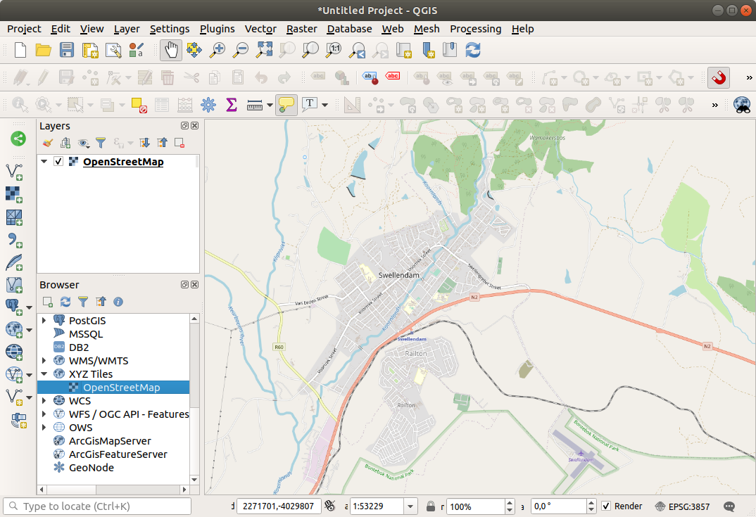
새로운 QGIS 프로젝트를 시작하십시오.
원하는 경우, 배경 맵을 추가해도 됩니다. Browser 를 열어서 XYZ Tiles 메뉴로부터 OSM 배경 맵을 불러오십시오.
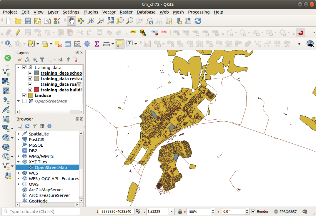
training_data.gpkgGeopackage 데이터베이스 파일에서, 이 수업에서 사용할 데이터셋 대부분을 찾을 수 있을 겁니다:buildingsroadsrestaurantsschools
이 데이터셋들과, 또
landuse.sqlite파일도 불러오십시오.남아프리카 공화국 Swellendam 시를 보려면 레이어 범위로 확대/축소하십시오.
Before proceeding we will filter the
roadslayer, in order to have only some specific road types to work with.오픈스트리트맵 데이터셋에 있는 도로 가운데 일부는
unclassified,tracks,path및footway로 목록화되어 있습니다. 우리는 이 예제에 더 적합한 다른 도로 유형들에 집중할 수 있도록 데이터셋에서 이들을 제외하고자 합니다.게다가, 모든 곳에서 오픈스트리트맵 데이터를 업데이트하지 못할 수도 있기 때문에
NULL값들도 제외할 것입니다.roads레이어를 오른쪽 클릭한 다음 Filter… 를 선택하십시오.대화창이 열리면 이 피처들을 다음 표현식으로 필터링합니다:
"highway" NOT IN ('footway', 'path', 'unclassified', 'track') AND "highway" IS NOT NULL
NOT과IN두 연산자를 연결해서 사용하면highway필드에 이 속성 값들을 가지고 있는 피처들을 모두 제외합니다.AND와IS NOT NULL두 연산자를 함께 사용하면highway필드에 어떤 값도 없는 도로들을 제외합니다.Note the
 icon next to the
 roadslayer. It helps you remember that this layer has a filter activated, so some features may not be available in the project.
모든 데이터를 불러온 맵은 다음 그림처럼 보일 것입니다:
6.2.5. ★☆☆ 혼자서 해보세요: 레이어 좌표계 변환하기
레이어들 안에서 거리를 측정할 것이기 때문에, 레이어의 좌표계를 변경해야 합니다. 이를 위해 각 레이어를 차례로 선택해서 새 투영체를 적용한 새 레이어로 저장한 다음 맵에 새 레이어를 가져와야 합니다.
서로 다른 옵션들이 많이 있습니다. 예를 들면, 각 레이어를 ESRI 셰이프파일 포맷 데이터셋으로 내보낼 수도 있고, 레이어들을 기존 GeoPackage 파일에 첨부할 수도 있고, 또는 또다른 GeoPackage 파일을 생성해서 새 재투영 레이어들로 채울 수도 있습니다. 여기에서는 training_data.gpkg 파일이 변경되지 않도록 마지막 옵션을 배워볼 것입니다. 여러분 자신에게 가장 적합한 워크플로를 선택하도록 하세요.
참고
이 예제에서는 WGS 84 / UTM zone 34S 좌표계를 사용하고 있지만, 여러분은 여러분의 지역에 더 적합한 UTM 좌표계를 사용해야 합니다.
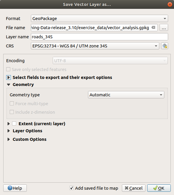
Right click the
roadslayer in the Layers panelExport –> Save Features As… 메뉴 항목을 클릭하십시오.
Save Vector Layer As 대화창에서 Format 으로 GeoPackage 를 선택하십시오.
File name 란 옆에 있는 … 버튼을 클릭하고 새 GeoPackage의 이름을
vector_analysis라고 입력하십시오.Layer name 을
roads_34S로 변경하십시오.CRS 를 WGS 84 / UTM zone 34S 로 변경하십시오.
OK 를 클릭하십시오:
이렇게 하면 새 GeoPackage 데이터베이스를 생성하고
roads_34S레이어를 추가할 것입니다.각 레이어에 대해 이 처리 과정을 반복하십시오.
vector_analysis.gpkgGeoPackage 파일에 새 레이어를 생성한 다음, 원본 이름 뒤에_34S를 붙이십시오.맥OS 상에서는, QGIS가 기존 GeoPackage를 덮어쓸 수 있도록 대화창에 있는 Replace 버튼을 누르십시오.
참고
기존 GeoPackage에 레이어를 저장한다고 선택한 경우, QGIS는 GeoPackage에 동일한 이름을 가진 레이어가 없는 한 GeoPackage에 있는 기존 레이어들 다음에 해당 레이어를 추가 할 것입니다.
프로젝트에서 예전 레이어들을 하나씩 제거하십시오.
모든 레이어에 대해 이 처리 과정을 완료하고 나면, 맵을 관심 지역으로 집중시키기 위해 레이어 가운데 하나를 오른쪽 클릭하고 Zoom to layer extent 메뉴를 클릭하십시오.
이제 오픈스트리트맵 데이터를 UTM 투영으로 변환했으니, 계산을 시작할 수 있습니다.
6.2.6. ★☆☆ 따라해보세요: 문제를 분석하기: 학교 및 도로부터의 거리
QGIS는 모든 벡터 객체 사이의 거리를 계산할 수 있습니다.
(작업 도중 맵을 단순화시키기 위해)
roads_34S와buildings_34S레이어만 가시화되어 있는지 확인하십시오.메뉴 항목을 클릭해서 QGIS의 분석 핵심 을 여십시오. 기본적으로 이 툴박스에서 (벡터 그리고 래스터 분석 용) 모든 알고리즘을 사용할 수 있습니다.
먼저 Buffer 알고리즘을 사용해서
roads_34S주변 지역을 계산합니다.:menuselection:Vector Geometry 그룹에서 버퍼 알고리즘을 찾을 수 있습니다.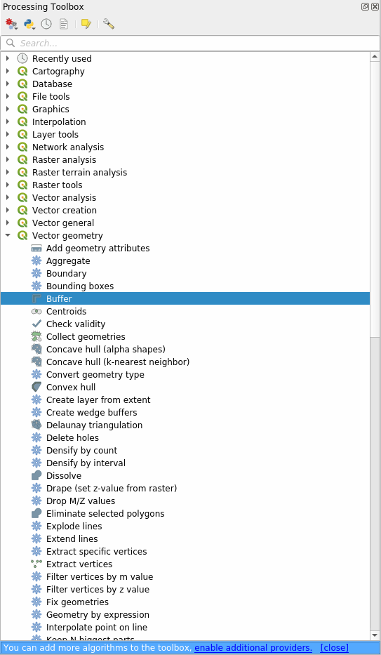
또는 툴박스의 상단에 있는 검색 메뉴에
buffer를 입력해도 됩니다: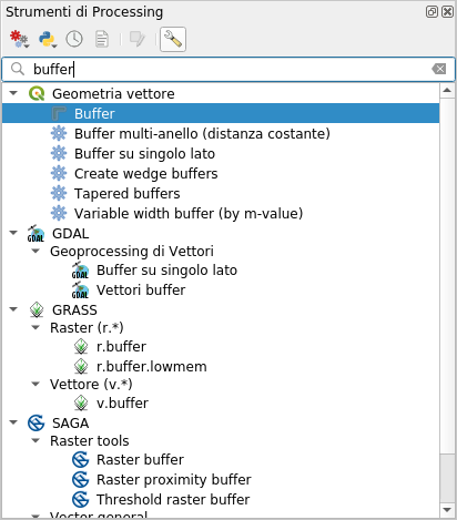
이 알고리즘을 더블 클릭하면 알고리즘 대화창이 열립니다.
Input layer 를
roads_34S로 선택하고 Distance 를 50으로 설정한 다음 나머지 파라미터들은 기본값으로 유지하십시오.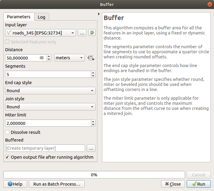
기본 Distance 는 미터 단위입니다. 입력 데이터셋이 미터를 기본 측정 단위로 사용하는 투영 좌표계이기 때문입니다. 킬로미터, 야드 등등의 다른 투영 단위를 선택하려면 콤보박스를 사용하면 됩니다.
참고
지리 좌표계인 레이어 상에 버퍼를 생성하려고 하는 경우, 공간 처리 프레임워크(Processing Framework)가 경고하고 해당 레이어를 미터법 좌표계로 재투영하라고 권고할 것입니다.
기본적으로, 공간 처리 프레임워크는 임시 레이어를 생성해서 Layers 패널에 추가합니다. GeoPackage 데이터베이스에 결과물을 다음과 같은 방법으로 첨부할 수도 있습니다:
… 버튼을 클릭한 다음 Save to GeoPackage… 메뉴를 선택하십시오.
새 레이어의 이름을
roads_buffer_50m으로 입력하십시오.vector_analysis.gpkg파일에 새 레이어를 저장하십시오.
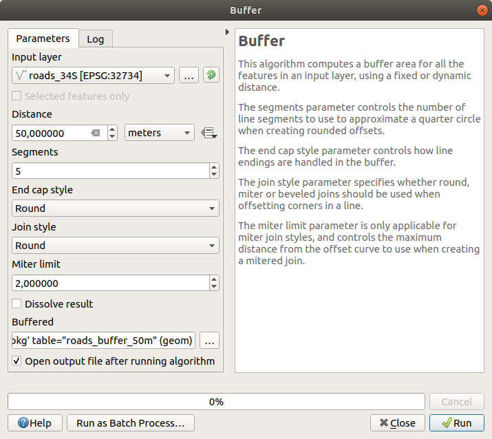
Run 버튼을 클릭한 다음, Buffer 대화창을 닫으십시오.
이제 여러분의 맵이 다음처럼 보일 것입니다:
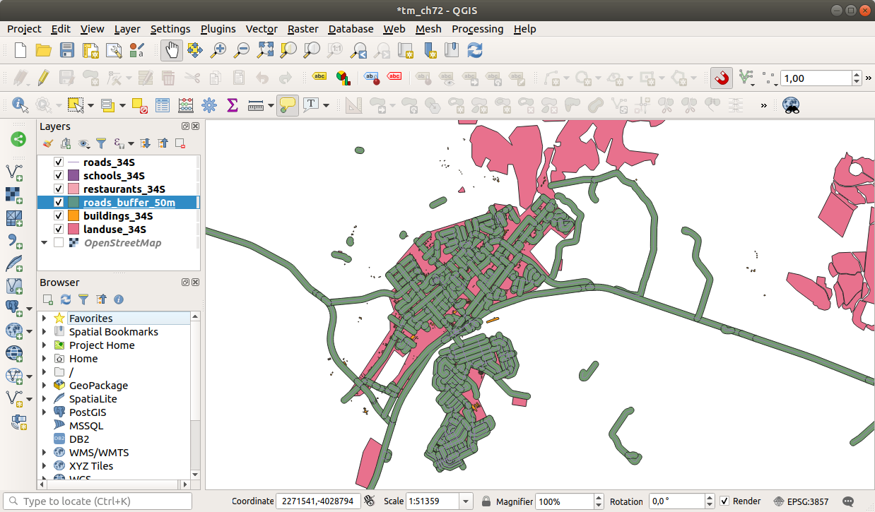
새 레이어가 Layers 목록 맨 위에 있는 경우, 맵을 많이 가릴 테지만 여러분의 지역에서 도로에서 50미터 이상 떨어져 있지 않은 모든 지역을 볼 수 있습니다.
이 버퍼 안에 개별 영역들이 있는 것이 보이십니까? 개별 도로 각각에 대응하는 버퍼들입니다. 이 문제를 해결하려면:
Uncheck the
roads_buffer_50mlayer and re-create the buffer with Dissolve results enabled.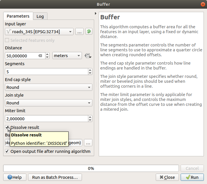
Save the output as
roads_buffer_50m_dissolvedRun 버튼을 클릭한 다음, Buffer 대화창을 닫으십시오.
Layers 패널에 이 레이어가 추가되고 나면 다음과 같이 보일 것입니다:
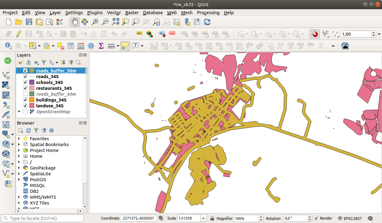
이제 필요 없는 부분들이 사라졌습니다.
참고
대화창의 오른쪽에 있는 짧은 도움말(Short Help) 은 알고리즘이 어떻게 작동하는지를 설명합니다. 더 자세한 정보가 필요한 경우, 대화창 하단에 있는 Help 버튼을 클릭하면 좀 더 자세한 알고리즘 지침이 열립니다.
6.2.7. ★☆☆ 혼자서 해보세요: 학교로부터의 거리
앞 단계와 동일한 방법으로 학교를 중심으로 하는 버퍼를 생성하십시오.
반경을 1 km 로 설정해야 합니다. vector_analysis.gpkg 파일에 새 레이어를 schools_buffer_1km_dissolved 로 저장하십시오.
해답
버퍼 대화창이 다음과 같이 보여야 합니다:
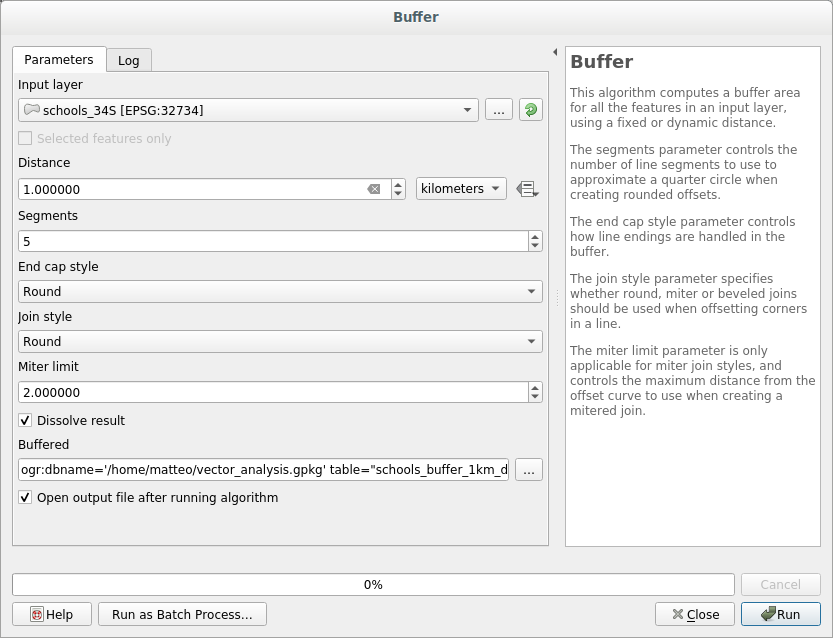
The Buffer distance is 1 kilometer.
The Segments to approximate value is set to
20. This is optional, but it’s recommended, because it makes the output buffers look smoother. Compare this: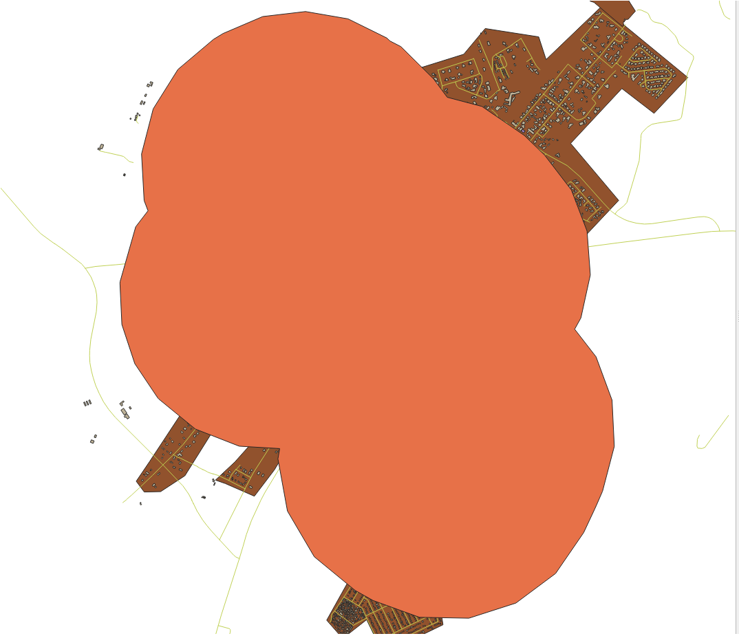
다음과 비교해보세요:
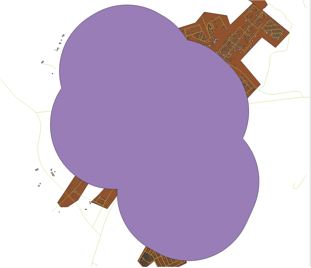
The first image shows the buffer with the Segments to approximate
value set to 5 and the second shows the value set to 20.
In our example, the difference is subtle, but you can see that the buffer’s edges
are smoother with the higher value.
6.2.8. ★☆☆ 따라해보세요: 중첩하는 영역들
이제 도로에서 50미터 이상 떨어져 있지 않은 지역과 학교에서 (도로 거리가 아니라 직선 거리로) 1킬로미터 안에 있는 지역을 식별했습니다. 그러나 당연하게도, 이 두 기준을 모두 만족시키는 지역만 필요할 뿐입니다. 이를 위해 Intersect 도구를 사용해야 합니다. Processing Toolbox 의 그룹에서 이 도구를 찾을 수 있습니다.
이 두 버퍼 레이어들을 각각 Input layer 와 Overlay layer 로 지정하고, Intersection 을
vector_analysis.gpkgGeoPackage 파일로 그리고 Layer name 을road_school_buffers_intersect로 선택하십시오. 나머지는 제안하는 대로 (기본값으로) 유지하십시오.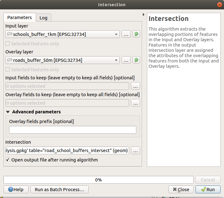
Run 을 클릭합니다.
다음 그림에서, 파란색 영역이 두 거리 기준을 모두 만족시키는 지역입니다.
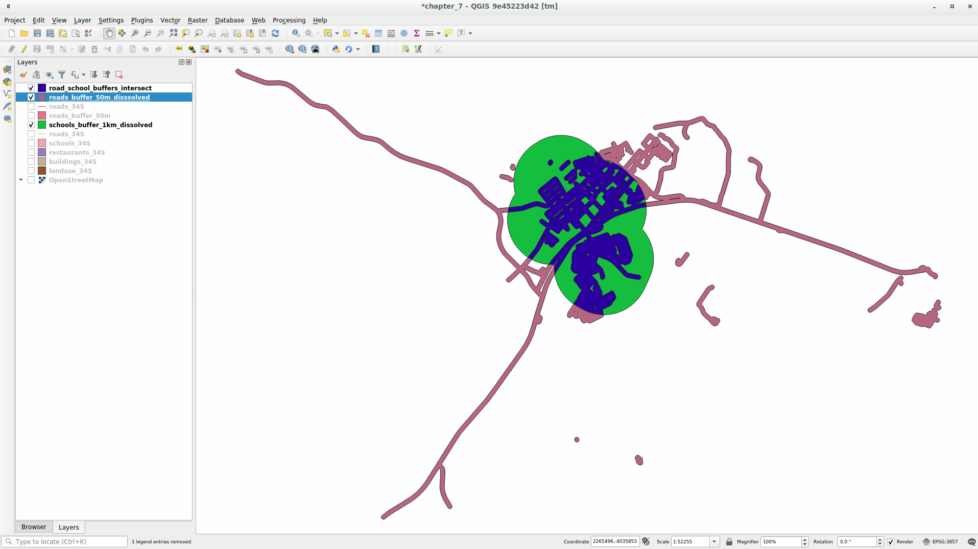
이제 두 버퍼 레이어를 제거하고 겹치는 구역만 보여주는 레이어만 남겨도 됩니다. 원래 그 레이어만을 원했기 때문입니다.
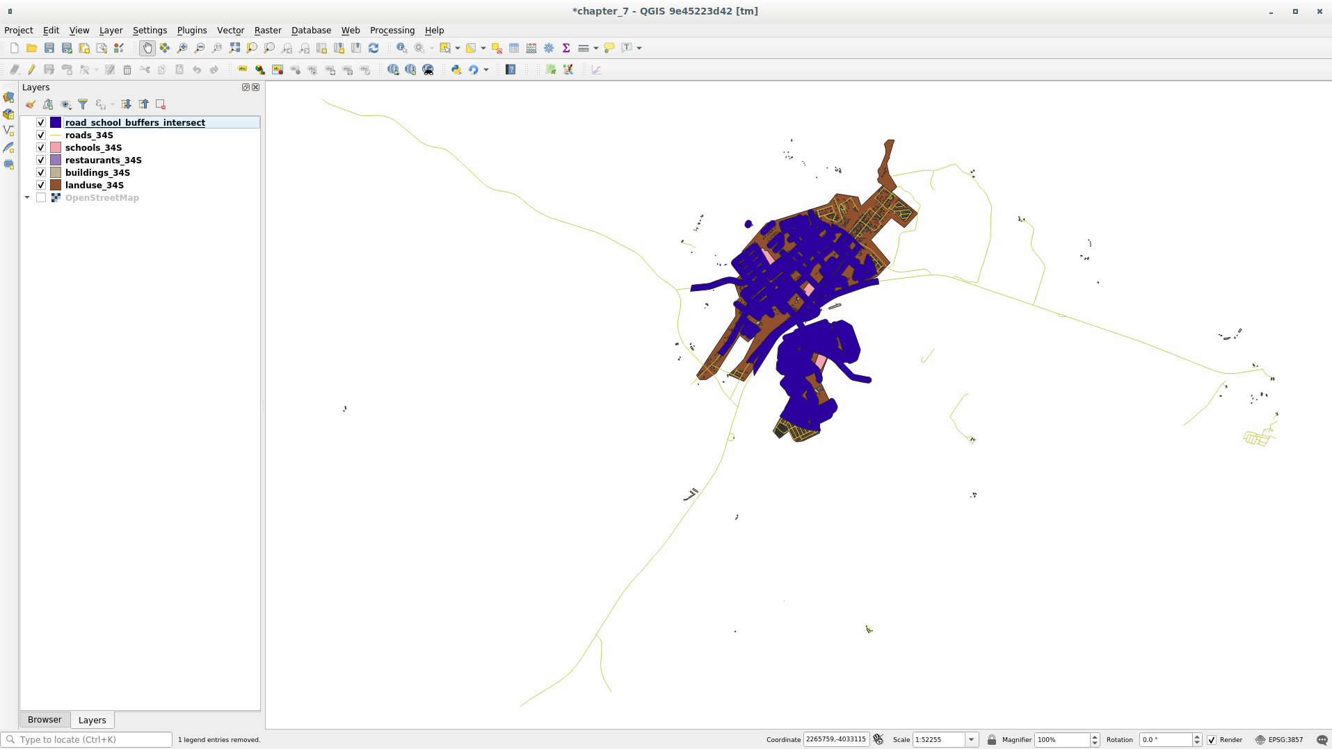
6.2.9. ★☆☆ 따라해보세요: 건물 추출하기
이제 건물들이 중첩해야만 하는 지역을 구했습니다. 다음은 해당 지역에 있는 건물들을 추출할 차례입니다.
Processing Toolbox 에서 메뉴 항목을 찾으십시오.
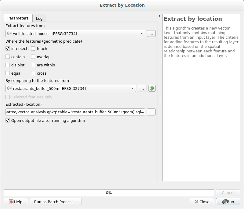
Extract features from 에
buildings_34S를 지정하십시오. Where the features (geometric predicate) 에서 intersect 를 체크하고, By comparing to the features from 에 버퍼 교차 영역 레이어를 선택하십시오.vector_analysis.gpkg파일에 이 레이어를well_located_houses라는 이름으로 저장하십시오.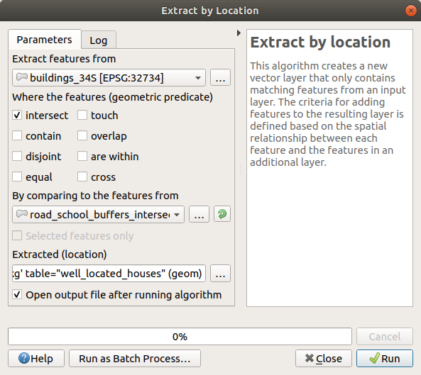
Run 버튼을 클릭한 다음 대화창을 닫으십시오.
You will probably find that not much seems to have changed. If so, move the
well_located_houseslayer to the top of the layers list, then zoom in.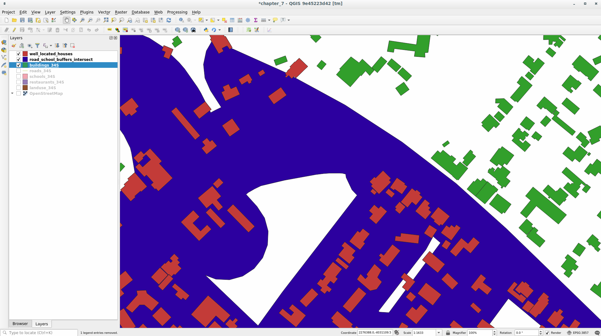
빨간색 건물들이 기준을 만족시키는 건물들이고, 초록색 건물들은 만족시키지 못하는 건물들입니다.
이제 개별 레이어 2개를 구했기 때문에 레이어 목록에서
buildings_34S를 제거해도 됩니다.
6.2.10. ★★☆ 혼자서 해보세요: 건물을 심화 필터링하기
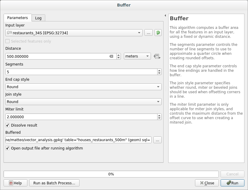
이제 학교에서 1km, 도로에서 50m 이내에 있는 모든 건물들을 보여주는 레이어가 생성됐습니다. 다음으로 이 레이어에서 식당으로부터 500m 이내에 있는 건물들만 추려내야 합니다.
Using the processes described above, create a new layer called
houses_restaurants_500m which further filters your
well_located_houses layer to show only those which are
within 500m of a restaurant.
해답
To create the new houses_restaurants_500m layer, we go through a two step
process:
먼저, 식당 주변에 500미터 버퍼를 생성한 다음 맵에 이 레이어를 추가하십시오:
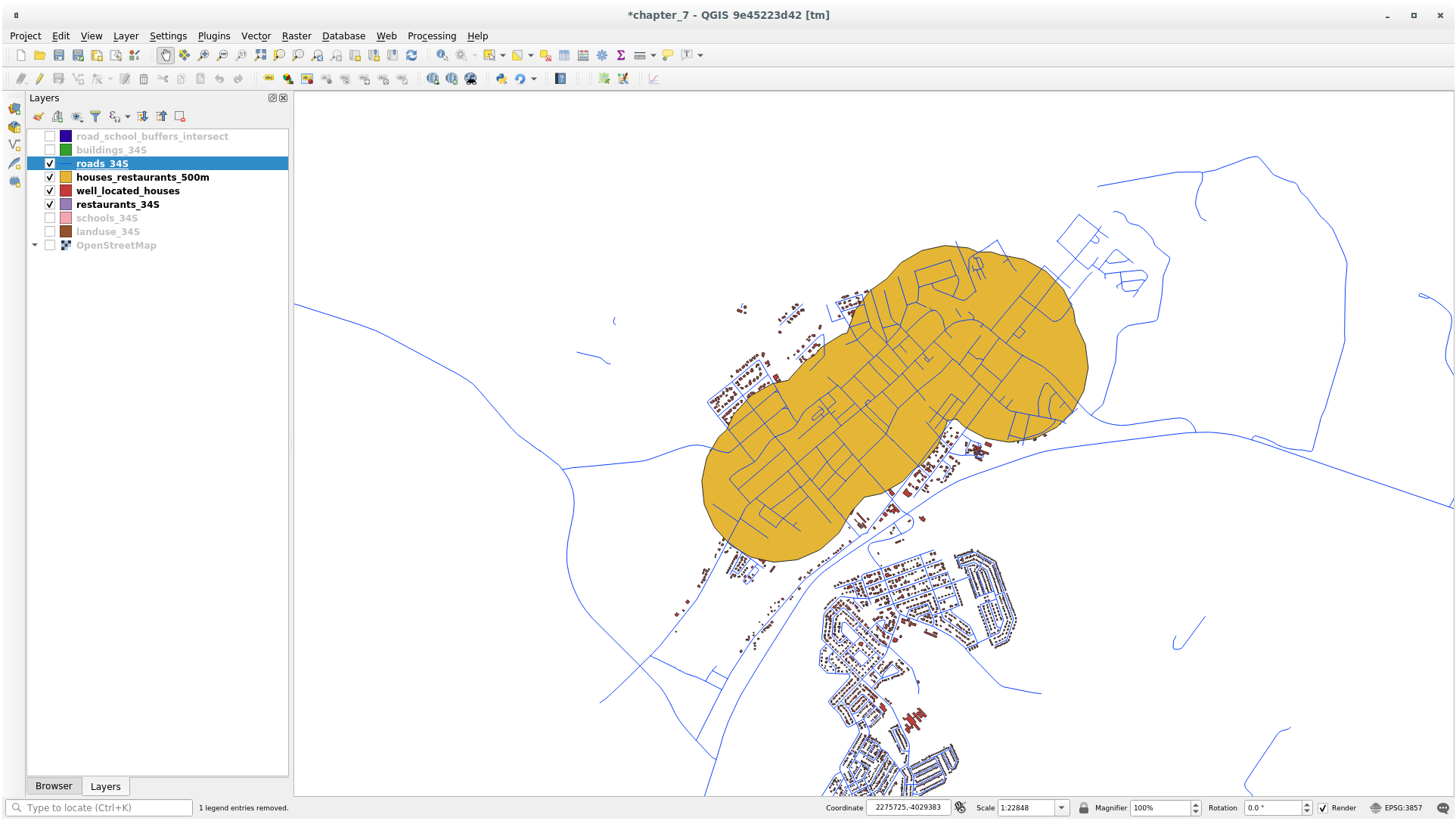
다음으로, 해당 버퍼 영역 안에 있는 건물들을 추출하십시오:
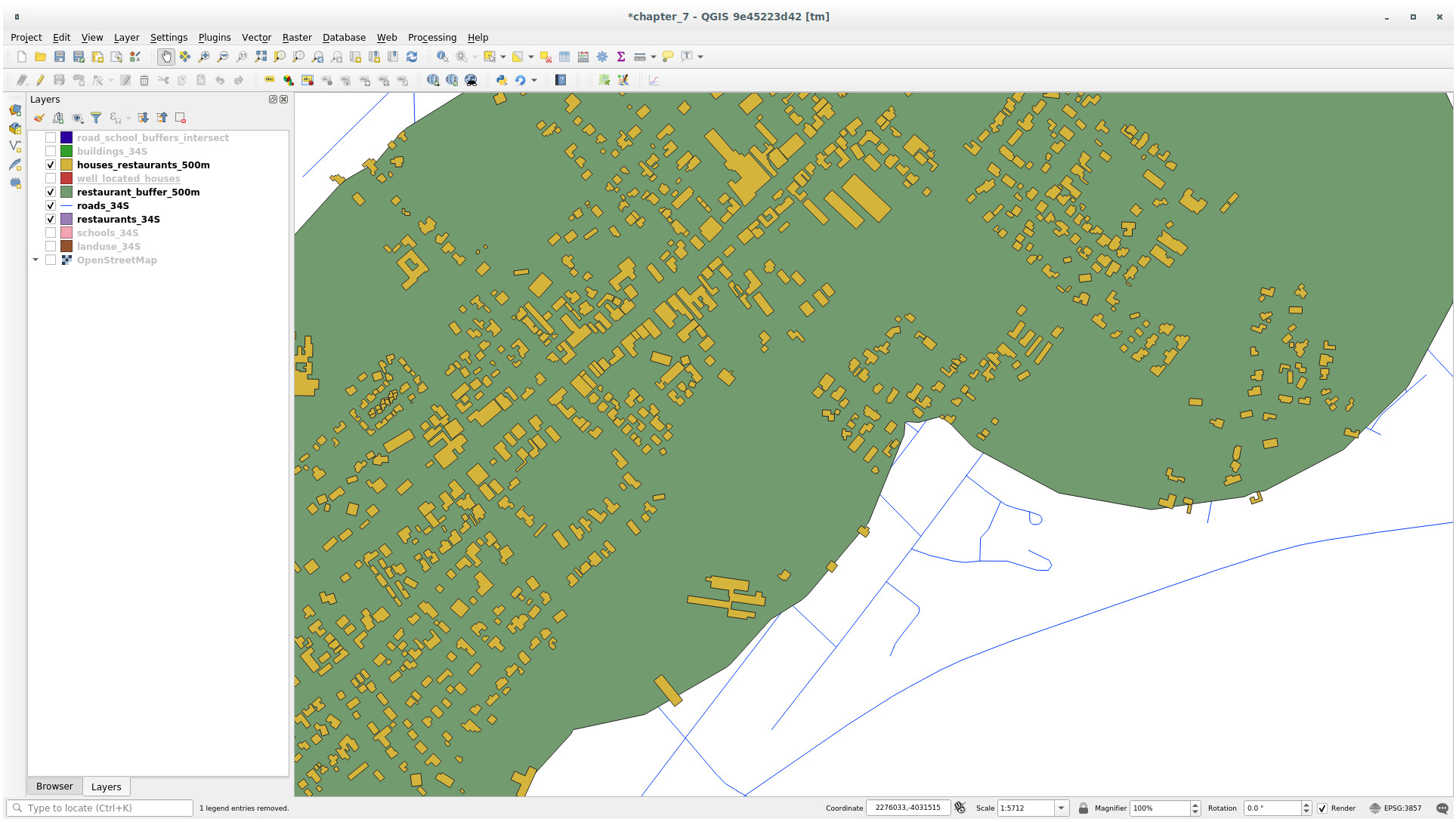
이제 여러분의 맵은 도로에서 50m, 학교에서 1km, 식당에서 500m 이내에 있는 건물들만 보여줄 것입니다:
6.2.11. ★☆☆ 따라해보세요: 알맞은 크기의 건물을 선택하기
어떤 건물이 정확한 면적인지 (100평방미터 이상인지) 보려면, 건물들의 면적을 계산해야 합니다.
Select the
houses_restaurants_500mlayer and open the Field Calculator by clicking on the Open Field Calculator button in the main toolbar or in
the attribute table window
Open Field Calculator button in the main toolbar or in
the attribute table windowCreate a new field 를 선택한 다음, Output field name 을
AREA로 설정하고 Output field type 을 Decimal number (real) 으로 선택하십시오. 마지막으로 그룹에서$area를 선택하십시오.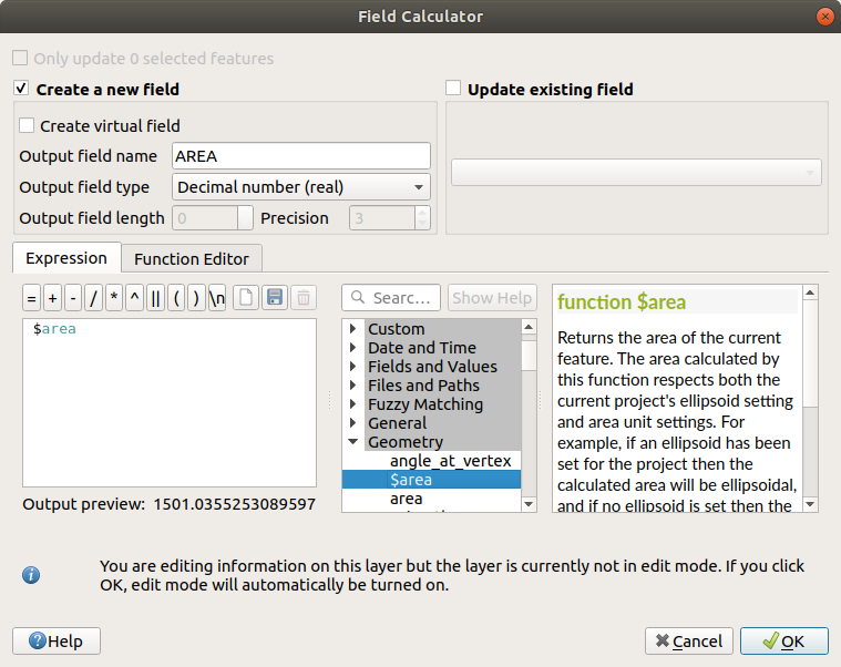
각 건물의 면적이 새
AREA필드에 평방미터 단위로 담기게 될 것입니다.OK 를 클릭합니다.
AREA필드가 속성 테이블 맨 끝에 추가되었습니다. Toggle Editing 버튼을 클릭해서 편집 작업을 완료하고, 메시지가 나타나면 편집 내용을 저장하십시오.
레이어 속성의 탭에서 Provider Feature Filter 를
"AREA" >= 100으로 설정하십시오.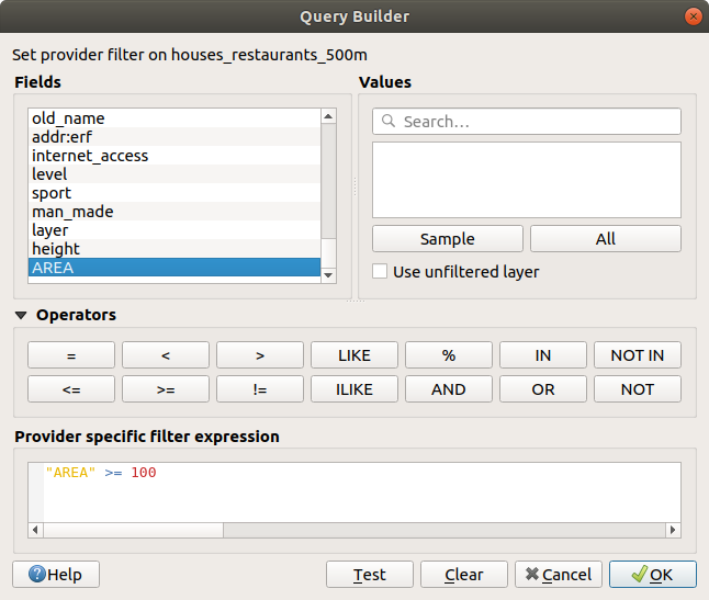
:guilabel:`OK`를 클릭하십시오.
이제 여러분의 맵에는 초기 기준을 만족시키면서 면적이 100평방미터 이상인 건물들만 보일 것입니다.
6.2.12. ★☆☆ 혼자서 해보세요:
앞에서 배웠던 접근법을 사용해서 여러분의 해답을 새 레이어로 저장하십시오. 이 파일은 동일한 GeoPackage 데이터베이스에 solution 이란 이름으로 저장해야 합니다.
6.2.13. 결론
GIS 문제 해결 접근법을 QGIS 벡터 분석 도구와 함께 사용해서 여러 기준을 가진 문제를 빠르고 쉽게 해결할 수 있었습니다.
6.2.14. 다음은 무엇을 배우게 될까요?
다음 수업에서는 어떤 포인트에서 다른 포인트까지 도로를 따르는 최단 거리를 계산하는 방법에 대해 알아볼 것입니다.