7.2. Lesson: 벡터 분석¶

7.2.1. GIS 처리 과정¶

시작하기 전 GIS 문제를 해결하는 데 사용할 수 있는 처리 과정을 간략히 살펴보는 것이 좋을 것입니다. 다음과 같은 처리 과정을 거칩니다.

1. 문제를 정의

2. 데이터 획득

3. 문제를 분석

4. 결과를 표출

7.2.2. The problem¶

해결해야 할 문제를 결정하는 것으로 처리 과정을 시작합시다. 예를 들어 여러분이 부동산 업자인데 다음 기준을 가진 고객을 위해 Swellendam 에 있는 거주지를 찾고 있다고 해봅시다.

1. It needs to be in Swellendam.
2. It must be within reasonable driving distance of a school (say 1km).
3. It must be more than 100m squared in size.
4. Closer than 50m to a main road.
5. Closer than 500m to a restaurant.

7.2.3. The data¶

이 문제들을 해결하려면 다음 데이터들이 필요합니다.

1. The residential properties (buildings) in the area.
2. The roads in and around the town.
3. The location of schools and restaurants.
4. The size of buildings.

All of this data is available through OSM and you should find that the dataset you have been using throughout this manual can also be used for this lesson. However, in order to ensure we have the complete data, we will re-download the data from OSM using QGIS’ built-in OSM download tool.

7.2.4. Follow Along: Start a Project¶

• Start a new QGIS project.
• Use the OpenStreetMap data download tool found in the Vector ‣ OpenStreetMap menu to download the data for your chosen region.
• Save the data as osm_data.osm in your exercise_data folder.
• Note that the osm format is a type of vector data. Add this data as a vector layer as usually Layer ‣ Add vector layer..., browse to the new osm_data.osm file you just downloaded. You may need to select Show All Files as the file format.
• Select osm_data.osm and click Open
• In the dialog which opens, select all the layers, except the other_relations and multilinestrings layer:

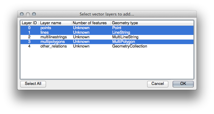
This will import the OSM data as separate layers into your map.

The data you just downloaded from OSM is in a geographic coordinate system, WGS84, which uses latitude and longitude coordinates, as you know from the previous lesson. You also learnt that to calculate distances in meters, we need to work with a projected coordinate system. Start by setting your project’s coordinate system to a suitable CRS for your data, in the case of Swellendam, WGS 84 / UTM zone 34S:

• Open the Project Properties dialog, select CRS and filter the list to find WGS 84 / UTM zone 34S.

• OK 를 클릭합니다.

We now need to extract the information we need from the OSM dataset. We need to end up with layers representing all the houses, schools, restaurants and roads in the region. That information is inside the multipolygons layer and can be extracted using the information in its Attribute Table. We’ll start with the schools layer:

• Right-click on the multipolygons layer in the Layers list and open the Layer Properties.
• Go to the General menu.
• Under Feature subset click on the [Query Builder] button to open the Query builder dialog.
• In the Fields list on the left of this dialog until you see the field amenity.
• Click on it once.
• Click the All button underneath the Values list:

Now we need to tell QGIS to only show us the polygons where the value of amenity is equal to school.

• Double-click the word amenity in the Fields list.
• Watch what happens in the Provider specific filter expression field below:

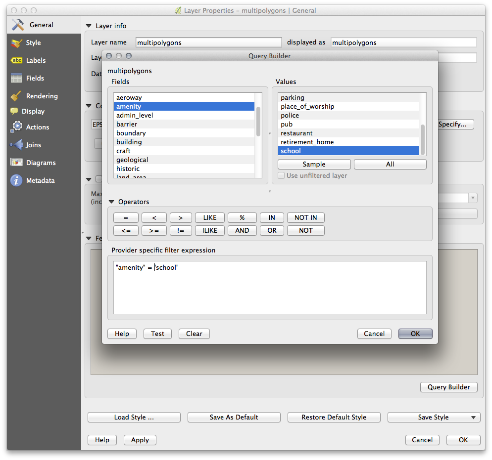
The word "amenity" has appeared. To build the rest of the query:

• Click the = button (under Operators).
• Double-click the value school in the Values list.
• Click OK twice.

This will filter OSM’s multipolygons layer to only show the schools in your region. You can now either:

• Rename the filtered OSM layer to schools and re-import the multipolygons layer from osm_data.osm, OR
• Duplicate the filtered layer, rename the copy, clear the Query Builder and create your new query in the Query Builder.

7.2.5. Try Yourself Extract Required Layers from OSM¶

Using the above technique, use the Query Builder tool to extract the remaining data from OSM to create the following layers:

• roads (from OSM’s lines layer)
• restaurants (from OSM’s multipolygons layer)
• houses (from OSM’s multipolygons layer)

You may wish to re-use the roads.shp layer you created in earlier lessons.

결과 확인

• Save your map under exercise_data, as analysis.qgs (this map will be used in future modules).
• In your operating system’s file manager, create a new folder under exercise_data and call it residential_development. This is where you’ll save the datasets that will be the results of the analysis functions.

7.2.6. Try Yourself Find important roads¶

Some of the roads in OSM’s dataset are listed as unclassified, tracks, path and footway. We want to exclude these from our roads dataset.

• Open the Query Builder for the roads layer, click Clear and build the following query:

  "highway"  != 'NULL' AND "highway" != 'unclassified' AND "highway" != 'track' AND "highway" != 'path' AND "highway" != 'footway'

You can either use the approach above, where you double-clicked values and clicked buttons, or you can copy and paste the command above.

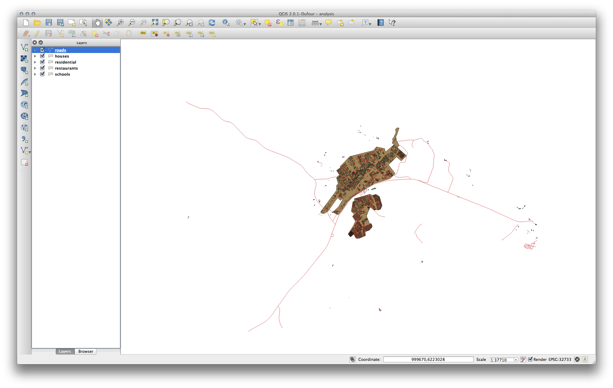
This should immediately reduce the number of roads on your map:

7.2.7. Try Yourself 레이어 CRS 변환¶

Because we are going to be measuring distances within our layers, we need to change the layers’ CRS. To do this, we need to select each layer in turn, save the layer to a new shapefile with our new projection, then import that new layer into our map.

• Right click the roads layer in the Layers panel.
• Click Save as...
• In the Save Vector As dialog, choose the following settings and click Ok (making sure you select Add saved file to map):

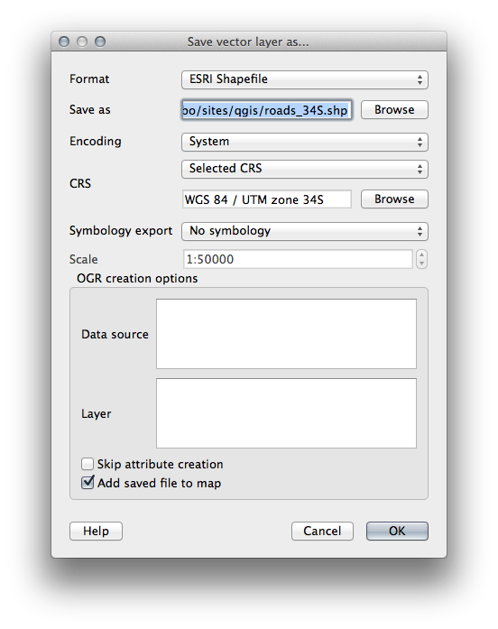
The new shapefile will be created and the resulting layer added to your map.

• Remove the old roads layer.

Repeat this process for each layer, creating a new shapefile and layer with “_34S” appended to the original name and removing each of the old layers.

각 레이어에 대해 이 과정을 완료한 다음 아무 레이어나 오른쪽 클릭하고 Zoom to layer extent 를 클릭해서 관심지역으로 맵을 이동시킵니다.

이제 OSM 데이터에 UTM 투영체를 적용시켰으니, 계산을 시작할 수 있습니다.

7.2.8. Follow Along: 문제 분석: 학교 및 도로부터의 거리¶

QGIS는 어떤 벡터 오브젝트부터의 거리도 계산할 수 있습니다.

• Make sure that only the roads_34S and houses_34S layers are visible, to simplify the map while you’re working.
• Click on the Vector ‣ Geoprocessing Tools ‣ Fixed distance buffer tool:

This gives you a new dialog.

• 다음과 같이 설정하십시오.

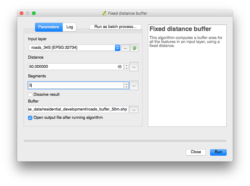
The Distance is in meters because our input dataset is in a Projected Coordinate System that uses meter as its basic measurement unit. This is why we needed to use projected data.

• Save the resulting layer under exercise_data/residential_development/ as roads_buffer_50m.shp.
• Click OK and it will create the buffer.
• When it asks you if it should “add the new layer to the TOC”, click Yes. (“TOC” stands for “Table of Contents”, by which it means the Layers list).
• Close the Fixed distance buffer dialog.

이제 여러분의 맵이 다음처럼 보일 것입니다.

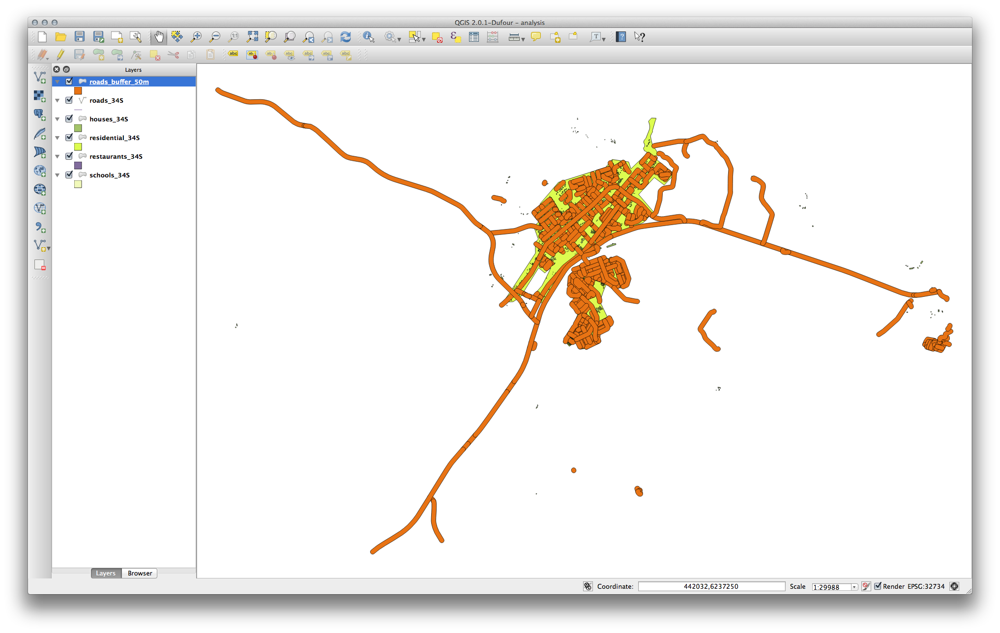
If your new layer is at the top of the Layers list, it will probably obscure much of your map, but this gives us all the areas in your region which are within 50m of a road.

However, you’ll notice that there are distinct areas within our buffer, which correspond to all the individual roads. To get rid of this problem, remove the layer and re-create the buffer using the settings shown here:

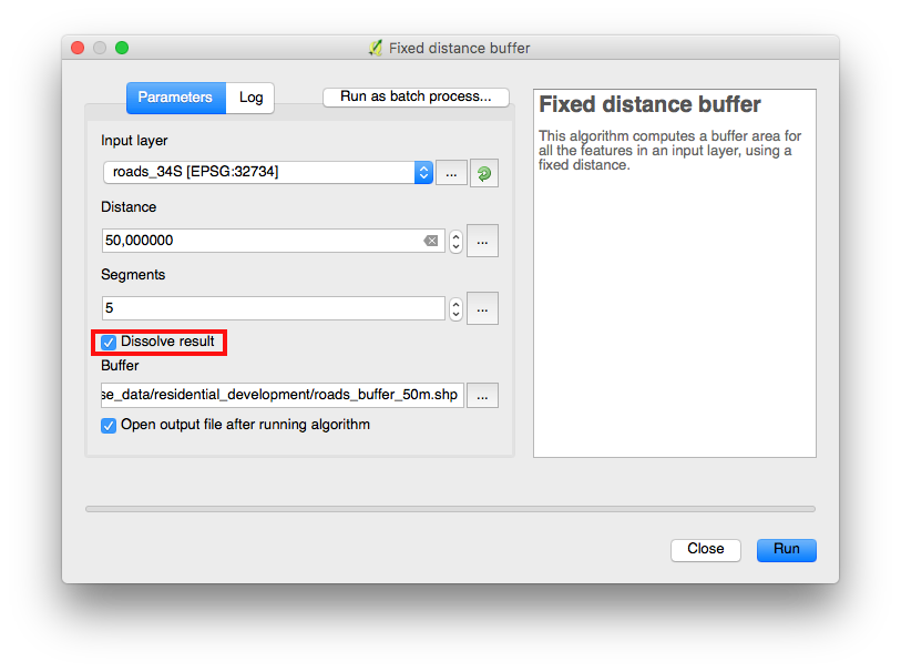
• Note that we’re now checking the Dissolve result box.
• Save the output under the same name as before (click Yes when it asks your permission to overwrite the old one).
• Click OK and close the Fixed distance buffer dialog again.

Once you’ve added the layer to the Layers list, it will look like this:

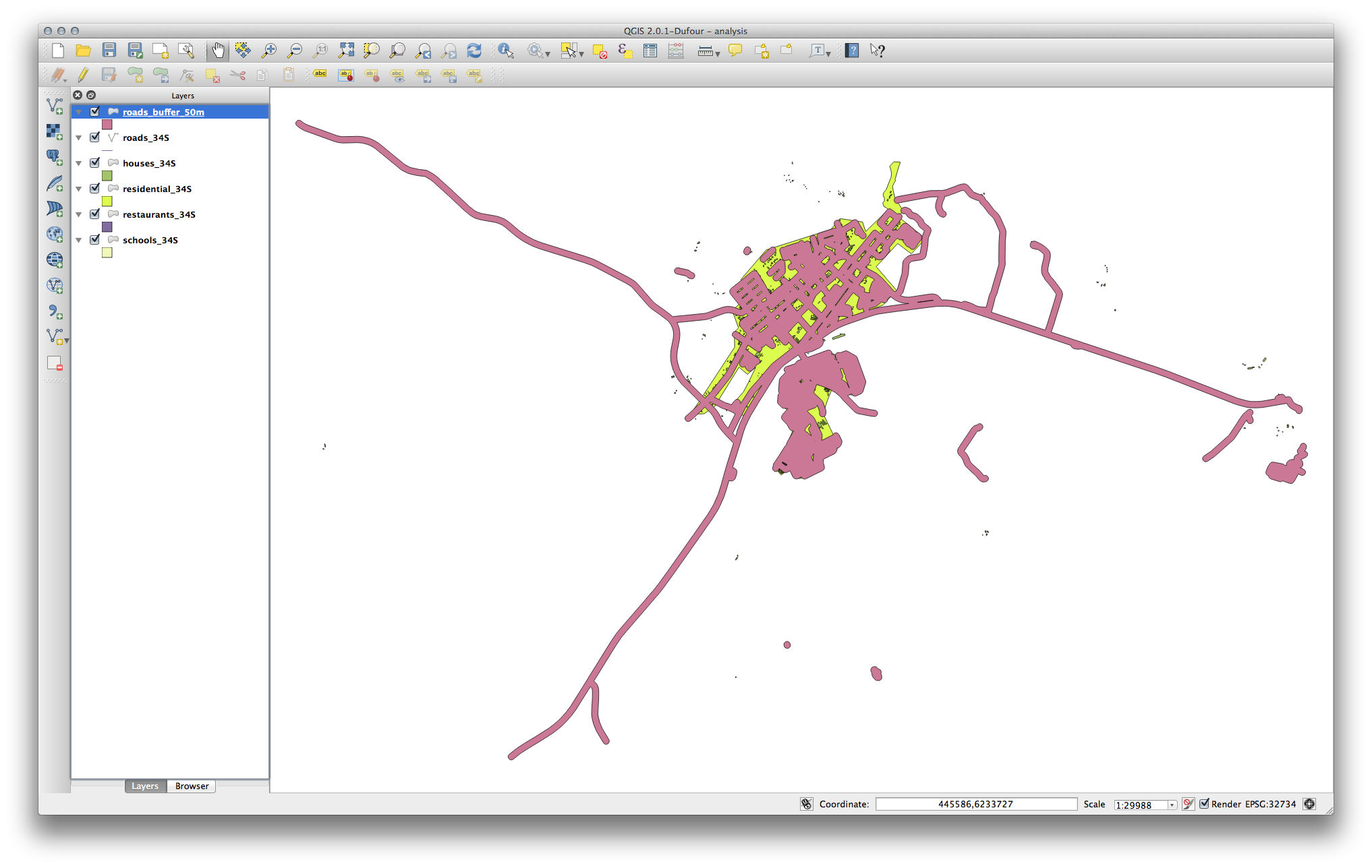
이제 필요 없는 부분들이 사라졌습니다.

7.2.9. Try Yourself 학교로부터의 거리¶

• 앞 단계와 동일한 방법으로 학교를 중심으로 하는 버퍼를 생성하십시오.

It needs to be 1 km in radius, and saved under the usual directory as schools_buffer_1km.shp.

결과 확인

7.2.10. Follow Along: 겹치는 구역¶

Now we have areas where the road is 50 meters away and there’s a school within 1 km (direct line, not by road). But obviously, we only want the areas where both of these criteria are satisfied. To do that, we’ll need to use the Intersect tool. Find it under Vector ‣ Geoprocessing Tools ‣ Intersect. Set it up like this:

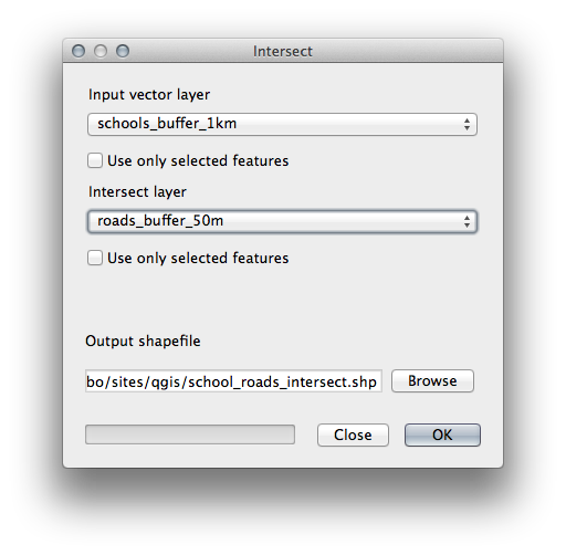
The two input layers are the two buffers; the save location is as usual; and the file name is road_school_buffers_intersect.shp. Once it’s set up like this, click OK and add the layer to the Layers list when prompted.

다음 이미지에서 두 가지 거리 기준을 모두 만족시키는 파란색 구역을 볼 수 있습니다!

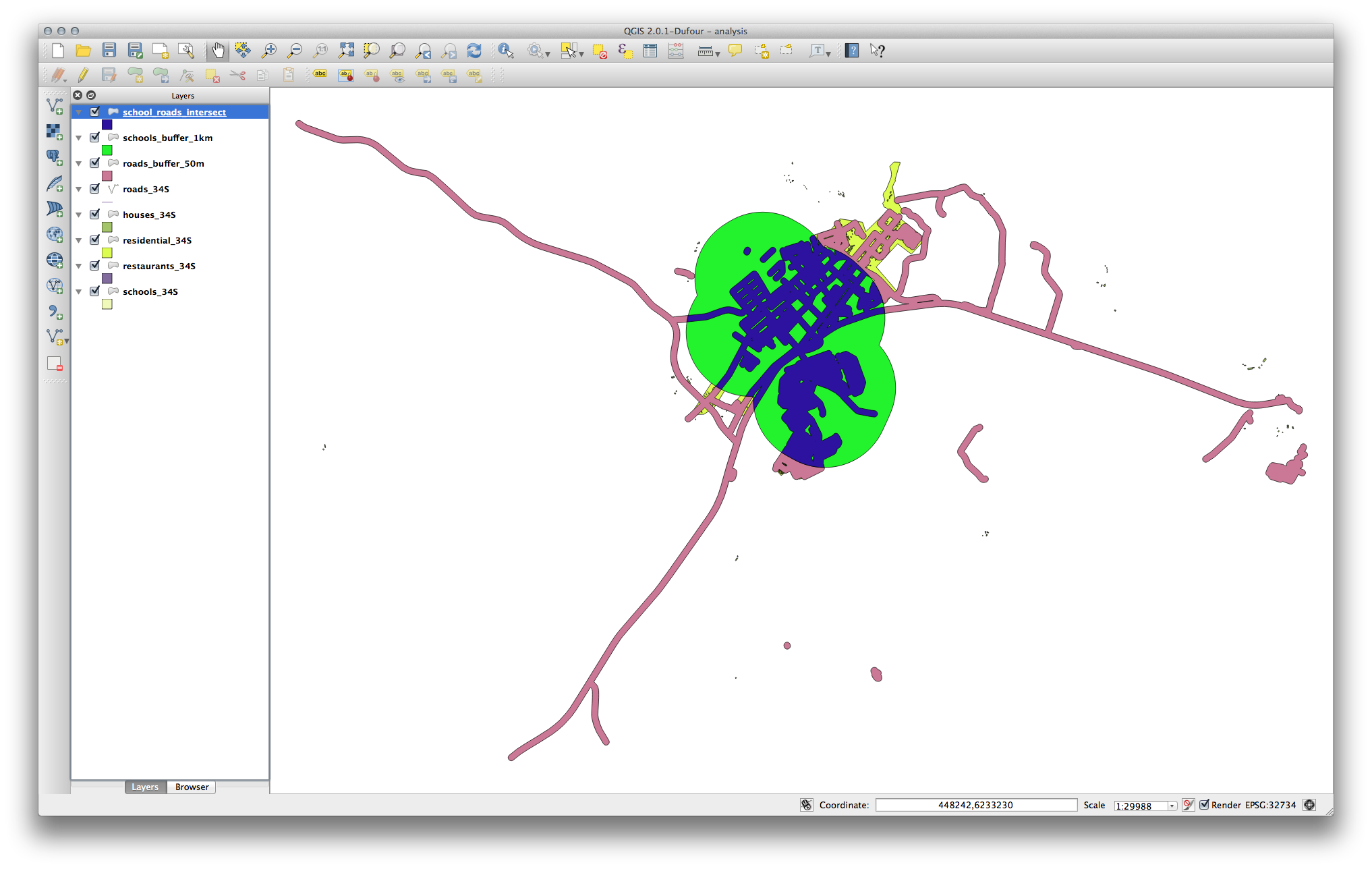
이제 두 버퍼 레이어를 제거하고 겹치는 구역만 보여주는 레이어만 남겨도 됩니다. 원래 그 레이어만을 원했기 때문입니다.

7.2.11. Follow Along: Select the Buildings¶

Now you’ve got the area that the buildings must overlap. Next, you want to select the buildings in that area.

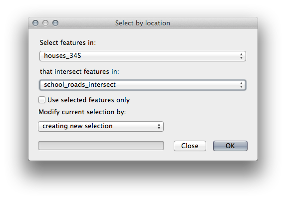
• Click on the menu entry Vector ‣ Research Tools ‣ Select by location. A dialog will appear.

• 다음과 같이 설정하십시오.

• Click OK, then Close.
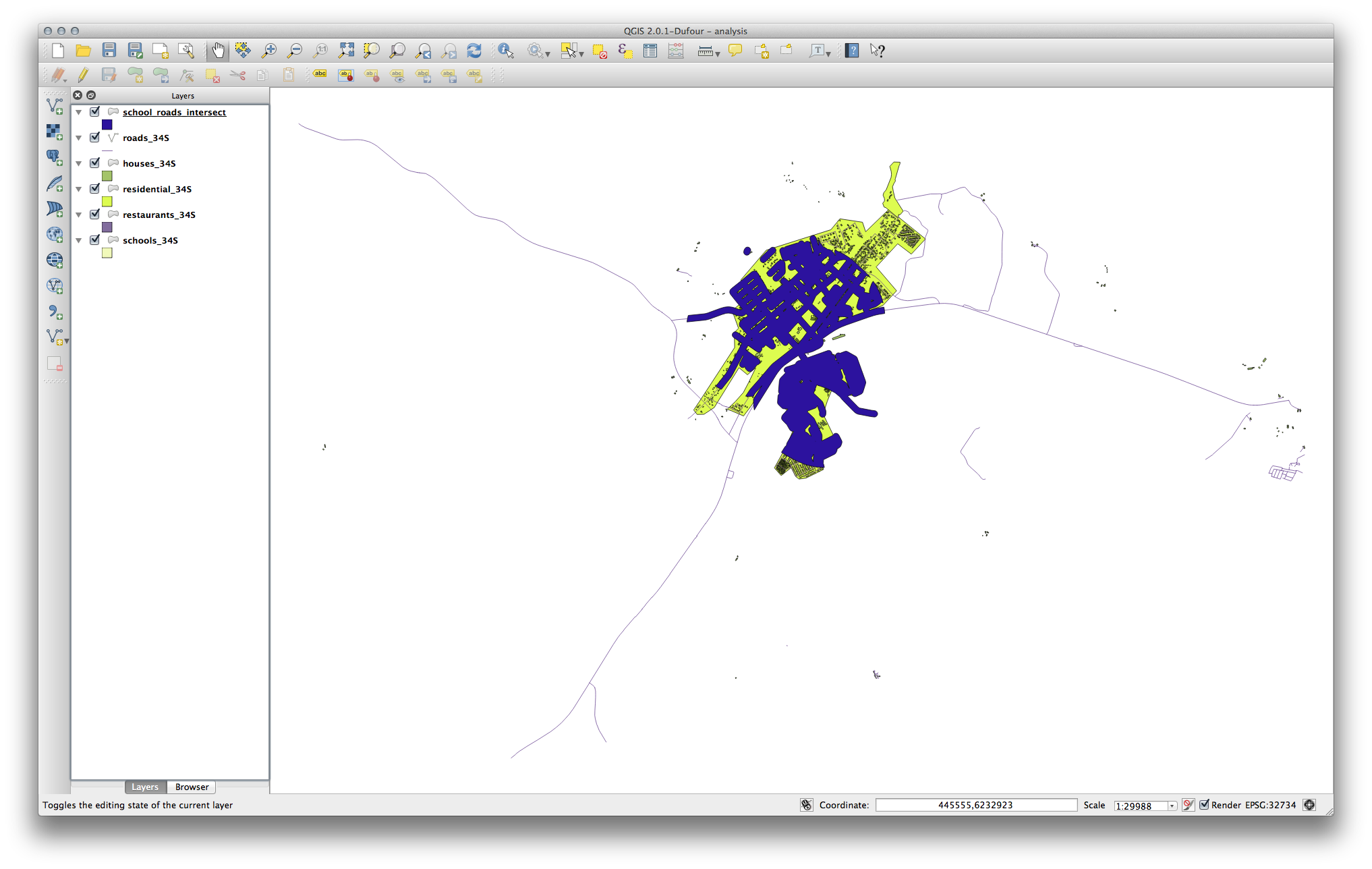
• You’ll probably find that not much seems to have changed. If so, move the school_roads_intersect layer to the bottom of the layers list, then zoom in:

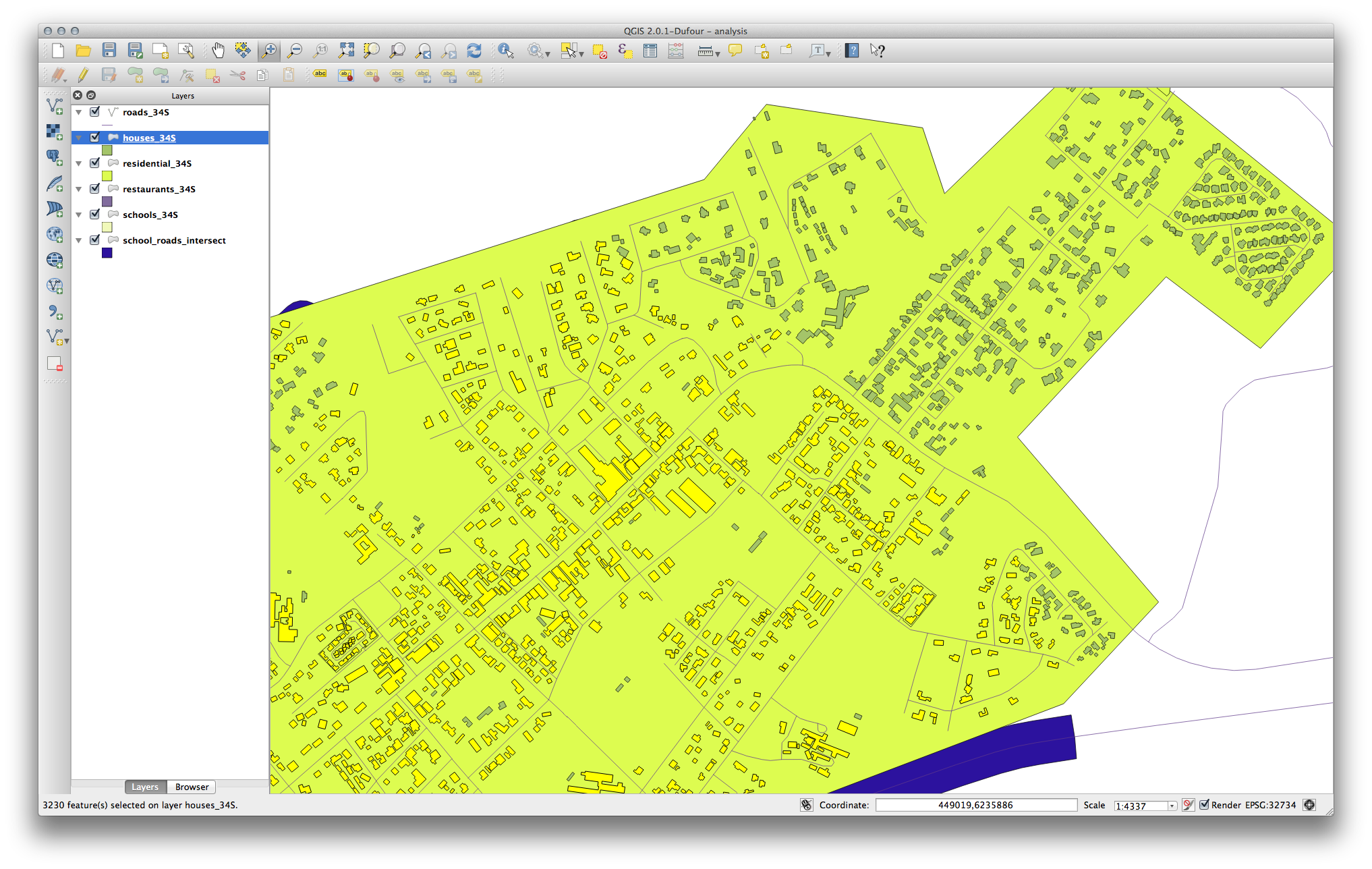
The buildings highlighted in yellow are those which match our criteria and are selected, while the buildings in green are those which do not. We can now save the selected buildings as a new layer.

• Right-click on the houses_34S layer in the Layers list.
• Select Save Selection As....
• Set the dialog up like this:

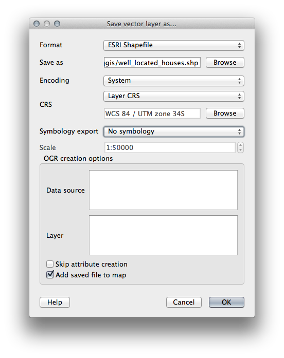
• The file name is well_located_houses.shp.

• OK 를 클릭합니다.

Now you have the selection as a separate layer and can remove the houses_34S layer.

7.2.12. Try Yourself 한 번 더 건물을 필터링¶

이제 학교에서 1km, 도로에서 50m 이내에 있는 모든 건물들을 보여주는 레이어가 생성됐습니다. 다음으로 이 레이어에서 식당으로부터 500m 이내에 있는 건물들만 추려내야 합니다.

Using the processes described above, create a new layer called houses_restaurants_500m which further filters your well_located_houses layer to show only those which are within 500m of a restaurant.

Check your results

7.2.13. Follow Along: 면적 기준을 만족하는 건물 선택¶

To see which buildings are the correct size (more than 100 square meters), we first need to calculate their size.

• Open the attribute table for the houses_restaurants_500m layer.
• Enter edit mode and open the field calculator.

• 다음과 같이 설정하십시오.

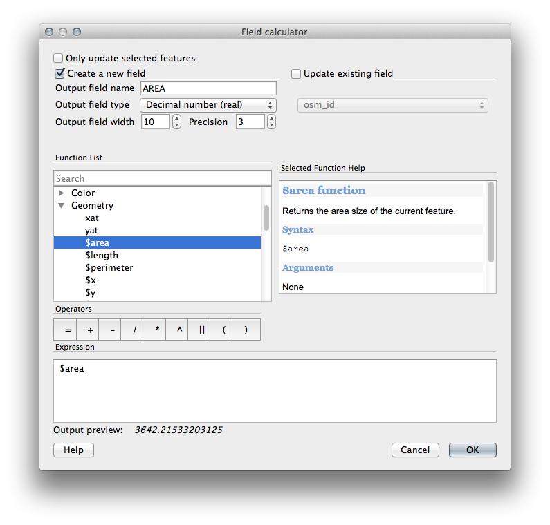
• If you can’t find AREA in the list, try creating a new field as you did in the previous lesson of this module.

• OK 를 클릭합니다.

• Scroll to the right of the attribute table; your AREA field now has areas in metres for all the buildings in your houses_restaurants_500m layer.

• 편집 모드 버튼을 한 번 더 클릭해서 편집을 끝내고, 편집 내용을 저장하십시오.

• Build a query as earlier in this lesson:

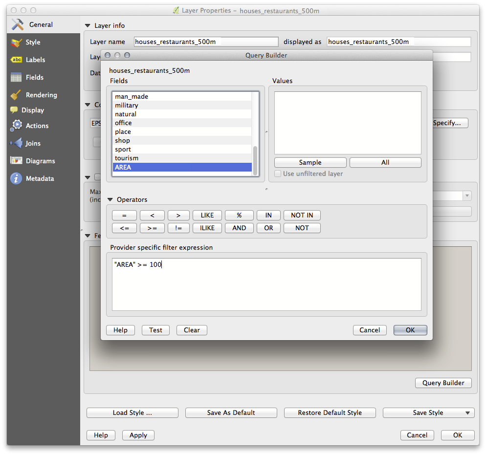
• Click OK. Your map should now only show you those buildings which match our starting criteria and which are more than 100m squared in size.

7.2.14. Try Yourself¶

• Save your solution as a new layer, using the approach you learned above for doing so. The file should be saved under the usual directory, with the name solution.shp.

7.2.15. In Conclusion¶

QGIS 벡터 분석 도구와 함께 GIS 문제 해결 접근법을 이용하면, 복합적인 기준을 가진 문제를 쉽고 빠르게 해결할 수 있습니다.

7.2.16. What’s Next?¶

다음 강의에서는 한 지점에서 다른 지점까지의 최단 거리를 도로를 따라 계산하는 방법을 배워보겠습니다.