7.1. Lesson: 데이터 재투영 및 변환¶

7.1.1. Follow Along: 투영¶

맵 자체는 물론 모든 데이터는 현재 WGS84라는 CRS를 사용하고 있습니다. WGS84는 데이터를 표현하는 데 쓰이는 매우 흔한 지리좌표계(GCS)입니다. 그러나 이제 곧 설명할 문제점도 가지고 있습니다.

• Save your current map.
• Then open the map of the world which you’ll find under exercise_data/world/world.qgs.
• Zoom in to South Africa by using the Zoom In tool.
• Try setting a scale in the Scale field, which is in the Status Bar along the bottom of the screen. While over South Africa, set this value to 1:5000000 (one to five million).
• Pan around the map while keeping an eye on the Scale field.

Notice the scale changing? That’s because you’re moving away from the one point that you zoomed into at 1:5000000, which was at the center of your screen. All around that point, the scale is different.

그 이유를 이해하려면, 지구의를 생각해보십시오. 남북 방향으로 선이 뻗어 있습니다. 이 경도 선들은 적도에서는 멀리 떨어져 있지만 남극/북극에서 만납니다.

GCS는 이 구체 상에서 정의되지만, 여러분의 모니터는 평면입니다. 평면에서 구체를 표현하려 할 때, 마치 테니스 공을 잘라서 평평하게 펼치려고 할 때처럼, 왜곡이 발생합니다. 즉 맵 상에서는 경도 선들이 (서로 만나야 할) 극지방에서도 평행하게 떨어져 있습니다. 다시 말해 맵 상에서 적도로부터 멀어질수록, 여러분이 보는 오브젝트의 축척이 점점 커진다는 뜻입니다. 한 마디로 말하자면 맵 상의 위치에 따라 축척이 계속 변한다는 말이지요!

이 문제를 해결하기 위해 투영좌표계(PCS)를 대신 사용해봅시다. PCS는 축척 변화를 감안하여 바로잡는 방식으로 데이터를 “투영”하거나 변환합니다. 따라서 축척을 일정하게 유지하려면 PCS를 이용해서 데이터를 재투영해야 합니다.

7.1.2. Follow Along: “실시간” 재투영¶

QGIS allows you to reproject data “on the fly”. What this means is that even if the data itself is in another CRS, QGIS can project it as if it were in a CRS of your choice.

• To enable “on the fly” projection, click on the CRS Status button in the Status Bar along the bottom of the QGIS window:

• In the dialog that appears, check the box next to Enable ‘on the fly’ CRS transformation.
• Type the word global into the Filter field. One CRS (NSIDC EASE-Grid Global) should appear in the list below.
• Click on the NSIDC EASE-Grid Global to select it, then click OK.

• 남아프리카 공화국의 형태가 어떻게 변하는지 보셨습니까? 투영체를 바꾸면 지구 상의 오브젝트의 형태가 바뀝니다.

• Zoom in to a scale of 1:5000000 again, as before.

• 맵을 이리저리 이동해보십시오.

• 축척이 일정하게 유지됩니다!

서로 다른 CRS를 이용하는 데이터셋을 결합하는 데에도 “실시간” 재투영을 사용할 수 있습니다.

• Deactivate “on the fly” re-projection again:
  • Click on the CRS Status button again.
  • Un-check the Enable ‘on the fly’ CRS transformation box.
  • Clicking OK.
• In QGIS 2.0, the ‘on the fly’ reprojection is automatically activated when layers with different CRSs are loaded in the map. To understand what ‘on the fly’ reprojection does, deactivate this automatic setting:
  • Go to Settings ‣ Options...
  • On the left panel of the dialog, select CRS.
  • Un-check Automatically enable ‘on the fly’ reprojection if layers have different CRS.
  • Click OK.
• Add another vector layer to your map which has the data for South Africa only. You’ll find it as exercise_data/world/RSA.shp.

보이십니까?

The layer isn’t visible! But that’s easy to fix, right?

• Right-click on the RSA layer in the Layers list.
• Select Zoom to Layer Extent.

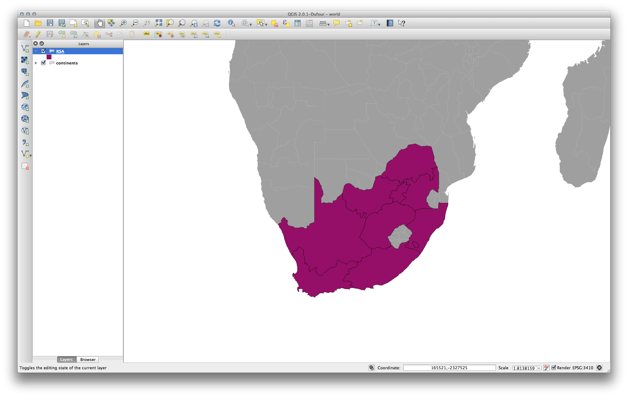
OK, so now we see South Africa... but where is the rest of the world?

It turns out that we can zoom between these two layers, but we can’t ever see them at the same time. That’s because their Coordinate Reference Systems are so different. The continents dataset is in degrees, but the RSA dataset is in meters. So, let’s say that a given point in Cape Town in the RSA dataset is about 4 100 000 meters away from the equator. But in the continents dataset, that same point is about 33.9 degrees away from the equator.

This is the same distance - but QGIS doesn’t know that. You haven’t told it to reproject the data. So as far as it’s concerned, the version of South Africa that we see in the RSA dataset has Cape Town at the correct distance of 4 100 000 meters from the equator. But in the continents dataset, Cape Town is only 33.9 meters away from the equator! You can see why this is a problem.

QGIS doesn’t know where Cape Town is supposed to be - that’s what the data should be telling it. If the data tells QGIS that Cape Town is 34 meters away from the equator and that South Africa is only about 12 meters from north to south, then that is what QGIS will draw.

To correct this:

• Click on the CRS Status button again and switch Enable ‘on the fly’ CRS transformation on again as before.
• Zoom to the extents of the RSA dataset.

Now, because they’re made to project in the same CRS, the two datasets fit perfectly:

When combining data from different sources, it’s important to remember that they might not be in the same CRS. “On the fly” reprojection helps you to display them together.

Before you go on, you probably want to have the ‘on the fly’ reprojection to be automatically activated whenever you open datasets having different CRS:

• Open again Settings ‣ Options... and select CRS.
• Activate Automatically enable ‘on the fly’ reprojection if layers have different CRS.

7.1.3. Follow Along: 다른 CRS로 데이터셋 저장¶

Remember when you calculated areas for the buildings in the Classification lesson? You did it so that you could classify the buildings according to area.

• Open your usual map again (containing the Swellendam data).
• Open the attribute table for the buildings layer.
• Scroll to the right until you see the AREA field.

Notice how the areas are all very small; probably zero. This is because these areas are given in degrees - the data isn’t in a Projected Coordinate System. In order to calculate the area for the farms in square meters, the data has to be in square meters as well. So, we’ll need to reproject it.

But it won’t help to just use ‘on the fly’ reprojection. ‘On the fly’ does what it says - it doesn’t change the data, it just reprojects the layers as they appear on the map. To truly reproject the data itself, you need to export it to a new file using a new projection.

• Right-click on the buildings layer in the Layers list.
• Select Save As... in the menu that appears. You will be shown the Save vector layer as... dialog.
• Click on the Browse button next to the Save as field.
• Navigate to exercise_data/ and specify the name of the new layer as buildings_reprojected.shp.
• Leave the Encoding unchanged.
• Change the value of the Layer CRS dropdown to Selected CRS.
• Click the Browse button beneath the dropdown.
• The CRS Selector dialog will now appear.
• In its Filter field, search for 34S.
• Choose WGS 84 / UTM zone 34S from the list.
• Leave the Symbology export unchanged.

The Save vector layer as... dialog now looks like this:

• Click OK.
• Start a new map and load the reprojected layer you just created.

Refer back to the lesson on Classification to remember how you calculated areas.

• Update (or add) the AREA field by running the same expression as before:

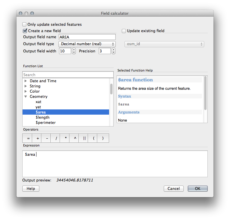
This will add an AREA field with the size of each building in square meters

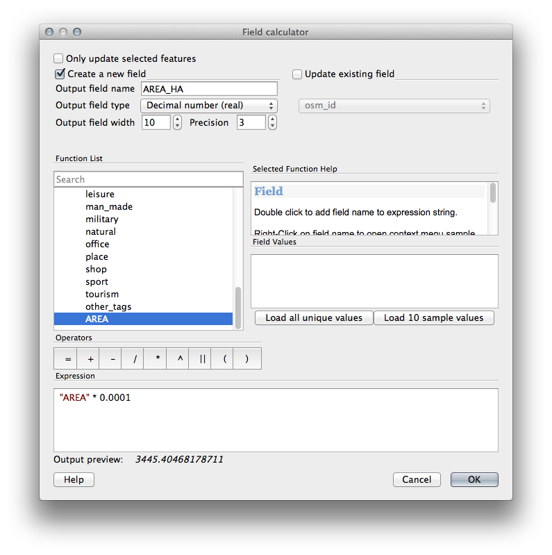
• To calculate the area in another unit of measurement, for example hectares, use the AREA field to create a second column:

Look at the new values in your attribute table. This is much more useful, as people actually quote building size in meters, not in degrees. This is why it’s a good idea to reproject your data, if necessary, before calculating areas, distances, and other values that are dependent on the spatial properties of the layer.

7.1.4. Follow Along: 사용자 지정 투영체 생성¶

QGIS에 기본으로 포함된 투영체 외에도 많은 투영체가 있습니다. 여러분 자신만의 투영체를 생성할 수도 있습니다.

• Start a new map.
• Load the world/oceans.shp dataset.
• Go to Settings ‣ Custom CRS... and you’ll see this dialog:

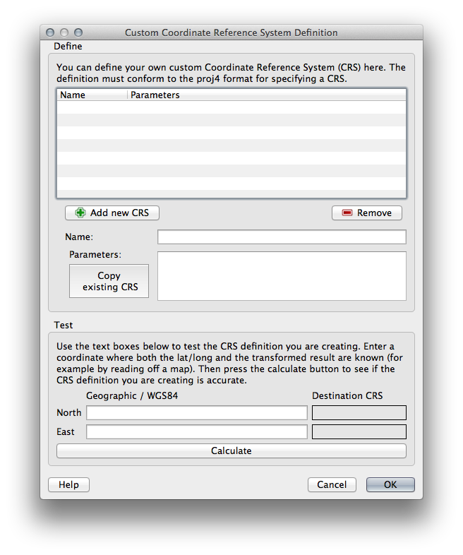
• Click on the Add new CRS button to create a new projection.

An interesting projection to use is called Van der Grinten I.

• Enter its name in the Name field.

이 투영체는 다른 대부분 투영체와는 달리 사각 면이 아니라 원형 면에 지구를 표현합니다.

• For its parameters, use the following string:

+proj=vandg +lon_0=0 +x_0=0 +y_0=0 +R_A +a=6371000 +b=6371000 +units=m +no_defs

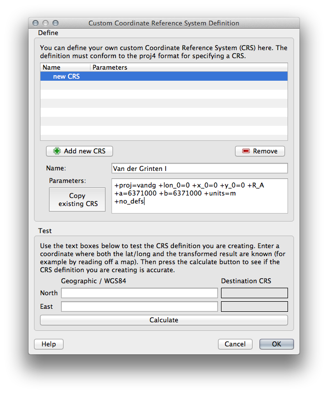
• Click OK.
• Enable “on the fly” reprojection.
• Choose your newly defined projection (search for its name in the Filter field).

• 이 투영체를 적용하면 맵이 다음과 같이 재투영될 것입니다.

7.1.5. In Conclusion¶

목적에 따라 유용한 투영체도 달라집니다. 올바른 투영체를 선택함으로써 사용자 맵 상에 피처를 정확하게 표현할 수 있게 됩니다.

7.1.6. Further Reading¶

Materials for the Advanced section of this lesson were taken from this article.

Further information on Coordinate Reference Systems is available here.

7.1.7. What’s Next?¶

다음 강의에서는 QGIS의 다양한 벡터 분석 도구들을 이용해 벡터 데이터를 분석하는 방법에 대해 배워보겠습니다.