중요
번역은 여러분이 참여할 수 있는 커뮤니티 활동입니다. 이 페이지는 현재 90.12% 번역되었습니다.
7.3. 수업: 지형 분석
래스터가 표현하고 있는 지형에 대해 더 깊이 이해할 수 있게 해주는 특정한 래스터 유형들이 있습니다. 수치표고모델(DEM)이 이런 점에서 특히 유용합니다. 이 수업에서는 지형 분석을 이용해서, 이전 강의에서 다뤘던 주거 구역 개발이라는 관점에서 이 연구 지역에 대해 더 자세히 알아보도록 하겠습니다.
이 수업의 목표: 지형 분석을 이용해서 지형에 대해 더 많은 정보를 끌어내기.
7.3.1. ★☆☆ 따라해보세요: 음영기복을 계산하기
이전 수업에서와 동일한 DEM 레이어를 사용할 것입니다. 이 수업을 아무 준비 없이 시작하는 경우, Browser 패널을 사용해서 raster/SRTM/srtm_41_19.tif 파일을 불러오십시오
DEM 레이어는 지형의 표고를 보여주지만, 조금 추상적으로 느껴질 때도 종종 있습니다. 여러분이 필요로 하는 지형에 대한 모든 3차원 정보를 담고 있지만 3차원 객체로 보이지는 않기 때문이죠. 이 지형에 대해 더 나은 인상을 받기 위해 음영기복(hillshade) 을 계산해볼 수 있습니다. 음영기복이란 3차원으로 보이는 이미지를 생성하기 위해 빛과 그림자를 사용한 지형을 매핑한 래스터를 말합니다.
메뉴에 있는 알고리즘들을 사용할 것입니다
메뉴를 클릭하십시오.
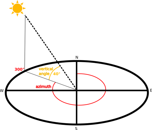
이 알고리즘은 광원의 위치를 지정할 수 있게 해줍니다: Azimuth 는 0(북쪽)에서 90(동쪽), 180(남쪽), 270(서쪽) 사이의 값을 가질 수 있는 반면, Vertical angle 은 광원이 얼마나 높이 있는지를 (0도에서 90도 사이의 값으로) 설정합니다.
다음 값들을 사용할 것입니다:
Z factor 는
1.0Azimuth (horizontal angle) 는
300.0°Vertical angle 은
40.0°
새로운
exercise_data/raster_analysis/폴더에 이 파일을hillshade.tif라는 이름으로 저장하십시오.마지막으로 Run 을 클릭하십시오.
You will now have a new layer called hillshade that looks like
this:
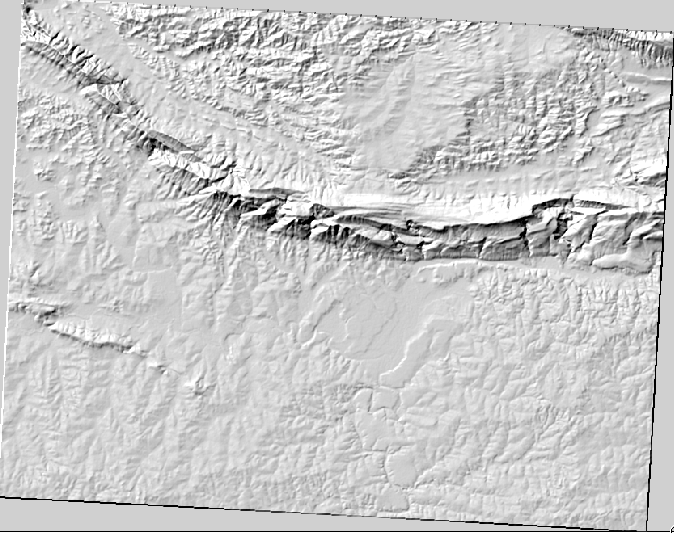
멋진 3D로 보입니다만, 좀 더 향상시킬 수는 없을까요? 음영기복도 그 자체로는 마치 석고 모형처럼 보입니다. 다른, 좀 더 다채로운 래스터들과 어떻게 함께 사용할 수는 없을까요? 물론 할 수 있습니다. 음영기복도를 오버레이로 사용한다면 말이죠.
7.3.2. ★☆☆ 따라해보세요: 음영기복도를 오버레이로 사용하기
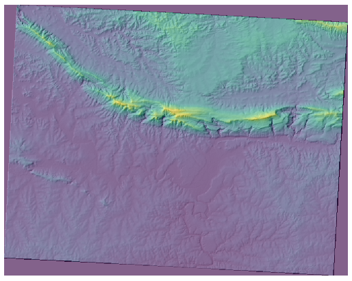
음영기복도는 낮 동안의 특정 시간의 햇빛에 대한 유용한 정보를 제공할 수 있습니다. 하지만 맵을 더 보기 좋게 하기 위한 심미적 목적을 위해서도 사용할 수 있습니다. 이렇게 하려면 음영기복도를 거의 투명하게 설정하면 됩니다.
Change the symbology of the original
srtm_41_19layer to use the Pseudocolor scheme as in the previous exerciseHide all the layers except the
srtm_41_19andhillshadelayersClick and drag the
srtm_41_19to be beneath thehillshadelayer in the Layers panelSet the
hillshadelayer to be transparent by clicking on the Transparency tab in the layer propertiesGlobal opacity 를
50%로 설정하십시오.결과는 다음과 같을 것입니다:
Switch the
hillshadelayer off and back on in the Layers panel to see the difference it makes.
Using a hillshade in this way, it’s possible to enhance the topography of the
landscape. If the effect doesn’t seem strong enough to you, you can change the
transparency of the hillshade layer; but of course, the brighter
the hillshade becomes, the dimmer the colors behind it will be. You will need
to find a balance that works for you.
작업 완료 시 프로젝트를 저장하는 것을 잊지 마세요.
7.3.3. 따라해보세요: 최적 지역 찾기
우리가 벡터 분석 수업에서 소개했던 부동산 업자 문제를 다시 생각해보십시오. 구매자들이 이제 건물을 구입해서 해당 부지에 작은 오두막을 짓고 싶어 한다고 상상해보죠. 남반구에서 이상적인 개발 도면은 다음과 같은 지역을 기반으로 해야 한다는 사실을 우리는 알고 있습니다:
북향
5도 미만의 경사
그러나 경사가 2도 미만인 경우, 경사 방향은 문제가 되지 않습니다.
이 기준을 만족시키는 최적 지역을 찾아봅시다.
7.3.4. ★★☆ 따라해보세요: 경사를 계산하기
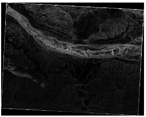
경사(slope) 는 지형이 얼마나 가파른지 알려줍니다. 예를 들어 해당 지형의 땅 위에 집을 짓는 경우, 상대적으로 평평한 땅이 필요할 것입니다.
경사를 계산하려면, 메뉴에 있는 알고리즘을 사용해야 합니다.
알고리즘을 여십시오.
Choose
srtm_41_19as the Elevation layerZ factor 는
1.0으로 유지하십시오.hillshade.tif와 같은 폴더에 산출 파일을slope.tif라는 이름으로 저장하십시오.Run 을 클릭하십시오.
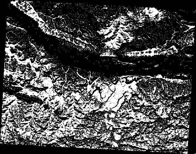
이제 각 픽셀이 해당하는 경사 값을 담고 있는 지형의 경사를 볼 수 있습니다. 지형이 평평할수록 픽셀이 검은색, 지형이 가파를수록 픽셀이 하얀색에 가까워집니다:
7.3.5. ★★☆ 혼자서 해보세요: 경사 방향을 계산하기
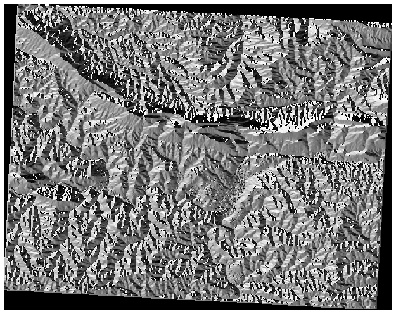
경사 방향(aspect) 이란 해당 지형의 경사가 바라보는 나침반 방향을 말합니다. 경사 방향이 0이면 경사가 북향이고, 90이면 동향, 180이면 남향, 270이면 서향이라는 뜻입니다.
연구 지역이 남반구에 존재하기 때문에, 건물이 햇빛을 받을 수 있으려면 북향 경사에 짓는 것이 이상적일 것입니다.
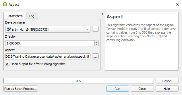
메뉴의 Aspect 알고리즘을 사용해서 slope.tif 와 같은 폴더에 aspect.tif 레이어를 저장하십시오.
해답
Aspect 대화창에서 다음과 같이 설정하십시오:
결과물은 다음과 같습니다:
7.3.6. ★★☆ 따라해보세요: 북쪽을 바라보는 경사 방향을 찾기
이제 경사는 물론 경사 방향도 보여주는 래스터들을 얻었지만, 이상적인 조건들을 한번에 만족시키는 곳을 알 도리가 없습니다. 이 분석은 어떻게 하는 것일까요?
그 답은 Raster calculator 가 가지고 있습니다.
QGIS는 서로 다른 래스터 계산기들을 제공합니다:
공간 처리에서:
각각의 도구는 동일한 결과를 내지만, 문법이 살짝 다를 수도 있고 사용할 수 있는 연산자들도 다를 수 있습니다.
우리는 공간 처리 툴박스 에 있는 를 사용할 것입니다.
래스터 계산기를 더블 클릭해서 여십시오.
대화창의 좌상단 부분에 불러온 모든 래스터 레이어들을
name@N으로 표현한 목록이 있습니다. 이때name은 레이어 이름이고N은 밴드 번호입니다.우상단 부분에서는 서로 다른 많은 연산자들이 보일 것입니다. 래스터가 이미지라는 사실을 잠깐 생각해보세요. 여러분은 래스터를 숫자로 채워진 2차원 행렬로 보아야 합니다.
북쪽은 0도이기 때문에, 북쪽을 바라보는 지형의 경우 그 경사 방향이 270도 이상이며 90도 이하여야 합니다. 따라서 공식은 다음과 같습니다:
aspect@1 <= 90 OR aspect@1 >= 270
이제 셀 크기, 범위 및 좌표계 같은 래스터 상세 정보를 설정해줘야 합니다. 직접 할 수도 있고
Reference layer를 선택함으로써 자동 설정할 수도 있습니다. Reference layer(s) 파라미터 옆에 있는 … 버튼을 클릭해서 후자를 선택하십시오.In the dialog, choose the
aspectlayer, because we want to obtain a layer with the same resolution.이 레이어를
aspect_north.tif로 저장하십시오.대화창이 다음과 같이 보여야 합니다.
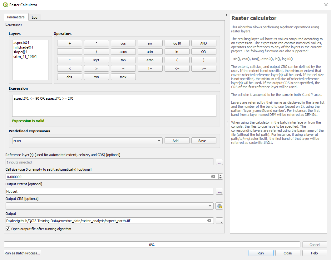
마지막으로 Run 을 클릭하십시오.
결과물이 다음과 같을 것입니다:
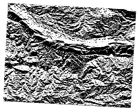
산출 값들은 0 또는 1 입니다. 이게 무슨 뜻일까요? 우리가 작성한 공식이 래스터에 있는 각 픽셀에 대해 해당 픽셀이 조건을 만족시키는지 아닌지를 반환합니다. 따라서 최종 결과물은 거짓 (0) 그리고 참 (1)이 되는 것입니다.
7.3.7. ★★☆ 혼자서 해보세요: 더 많은 기준들
이제 경사 방향 작업이 끝났으니, DEM으로부터 새 레이어 2개를 생성하십시오.
첫 번째 레이어는 경사가
2도 이하인 지역을 나타내야 합니다.두 번째 레이어도 비슷하지만, 경사가
5도 이하여야 합니다.exercise_data/raster_analysis디렉터리에 두 레이어를 각각slope_lte2.tif와slope_lte5.tif로 저장하십시오.
해답
Raster calculator 대화창에서 다음과 같이 설정하십시오:
표현식은 다음과 같습니다:
slope@1 <= 2Reference layer(s) 에
slope레이어를 선택합니다.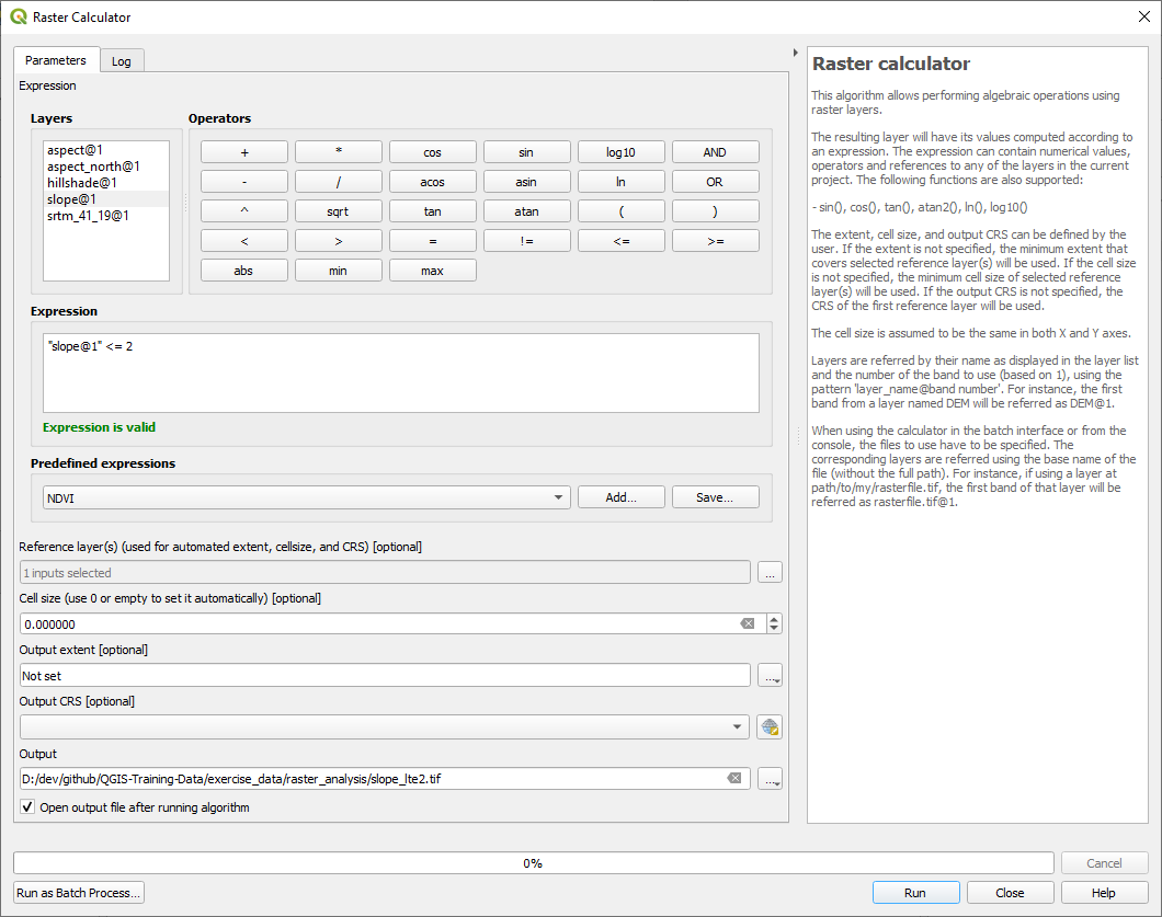
5도 버전의 경우, 표현식과 파일 이름의
2를5로 바꿉니다.
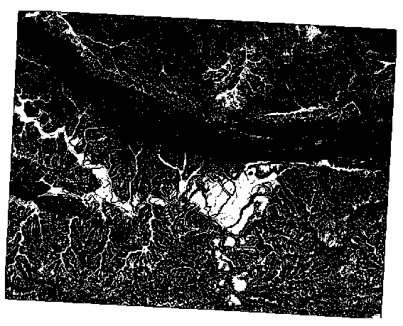
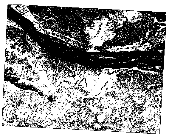
결과물은 다음과 같습니다:
2도:
5도:
7.3.8. ★★☆ 따라해보세요: 래스터 분석 결과들을 결합하기
이제 DEM으로부터 래스터 레이어 3개를 생성했습니다:
aspect_north: terrain facing northslope_lte2: slope equal to or below 2 degreesslope_lte5: slope equal to or below 5 degrees
조건을 만족시키는 장소의 픽셀 값은 1 입니다. 만족시키지 못하는 픽셀의 값은 0 입니다. 따라서 이 래스터들을 곱하면 모든 래스터에서 값이 1 인 픽셀의 값이 1 이 될 것입니다. (나머지 픽셀들의 값은 0 이 될 것입니다.)
만족시켜야 할 조건들은 다음과 같습니다:
경사가 5도 이하인 곳의 지형은 북향이어야만 합니다.
경사가 2도 이하인 곳은 지형이 바라보는 방향이 어느 쪽이든 상관없습니다.
따라서 경사가 5도 이하 AND 지형이 북향, OR 경사가 2도 이하인 지역을 찾아야 합니다. 이런 지형이 개발에 적합할 것입니다.
이 기준들을 만족시키는 지역을 계산하려면:
다시 Raster calculator 를 여십시오.
Expression 에 다음 표현식을 입력하십시오:
( aspect_north@1 = 1 AND slope_lte5@1 = 1 ) OR slope_lte2@1 = 1
Reference layer(s) 파라미터를
aspect_north로 설정하십시오. (다른 레이어를 선택해도 상관없습니다 — 모두srtm_41_19레이어로부터 계산된 레이어들이기 때문입니다.)exercise_data/raster_analysis/디렉터리에 산출 파일을all_conditions.tif로 저장하십시오.Run 을 클릭합니다.
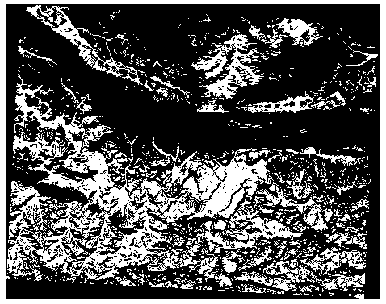
결과물은 다음과 같습니다:
힌트
다음 명령어를 사용하면 이전 단계들을 단순화시킬 수 있습니다:
((aspect@1 <= 90 OR aspect@1 >= 270) AND slope@1 <= 5) OR slope@1 <= 2
7.3.9. ★★☆ 따라해보세요: 래스터를 단순화시키기
앞의 이미지를 보면 알 수 있듯이, 결합된 분석의 결과물에서 조건들을 만족시키는 (하얀색) 지역들이 아주, 아주 작습니다. 그러나 이런 지역들은 실제 분석에 유용하지 않습니다. 무언가를 짓기에는 너무 작은 부지들이기 때문입니다. 이렇게 너무 작아서 사용할 수 없는 지역들을 모두 제거해봅시다.
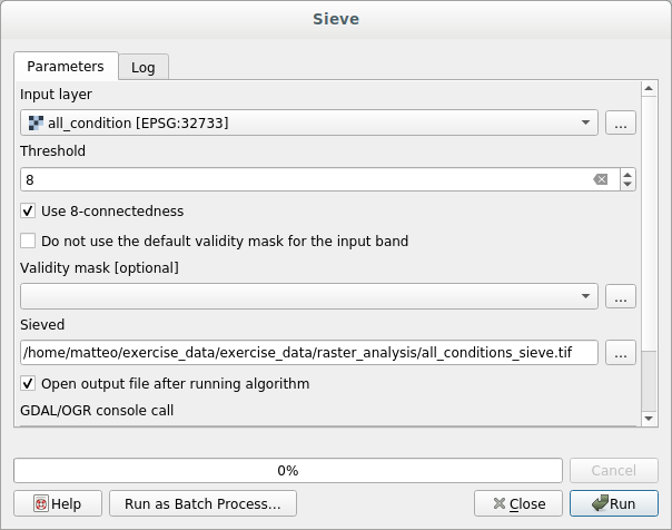
Sieve 도구를 여십시오. (Processing Toolbox 의 메뉴에 있습니다.)
Input file 을
all_conditions로, Sieved 를 (exercise_data/raster_analysis/아래)all_conditions_sieve.tif로 설정하십시오.Threshold 를 8로 (연속하는 픽셀을 최소 8개로) 설정하고, Use 8-connectedness 옵션을 체크하십시오.
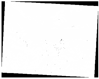
처리 과정이 완료되면 새 레이어를 불러올 것입니다.
무슨 일이 일어난 것일까요? 그 답은 새 래스터 파일의 메타데이터에 있습니다.
Layer Properties 대화창의 Information 탭에서 메타데이터를 검토해보십시오.
STATISTICS_MINIMUM값을 찾아보세요: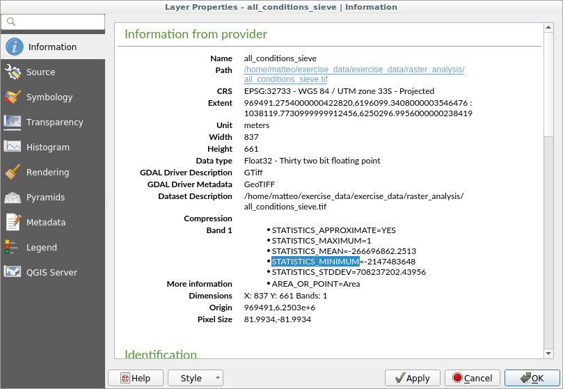
이 래스터는 이 래스터를 파생시킨 래스터와 같이
1과0값만 가지고 있어야 하지만, 매우 큰 음수도 가지고 있습니다. 데이터를 검토해보면 이 숫자가 NULL 값 역할을 한다는 사실을 알 수 있습니다. 필터링을 통과한 지역만 필요하기 때문에, 이 NULL 값들을 0으로 설정합시다.Raster Calculator 를 열어서 다음 표현식을 작성하십시오:
(all_conditions_sieve@1 <= 0) = 0
이 표현식은 음수가 아닌 값들을 모두 유지하고 음수들을 0으로 설정해서,
1값을 가진 지역들을 모두 온전히 유지할 것입니다.exercise_data/raster_analysis/디렉터리에 산출 파일을all_conditions_simple.tif로 저장하십시오.
산출물은 다음과 같습니다:
우리가 기대한 산출물입니다. 이전 결과물을 단순화시킨 버전이죠. 어떤 도구의 결과물이 예상했던 것과 다를 경우, 문제를 해결하는 데 메타데이터(그리고 적용할 수 있는 경우 벡터 속성)을 살펴보는 작업이 필수적일 수 있습니다.
7.3.10. ★★☆ 따라해보세요: 래스터를 재범주화하기
래스터 레이어에 대한 계산을 하기 위해 래스터 계산기 를 사용했습니다. 기존 레이어에서 정보를 추출하는 데 사용할 수 있는 강력한 도구가 또 있습니다.
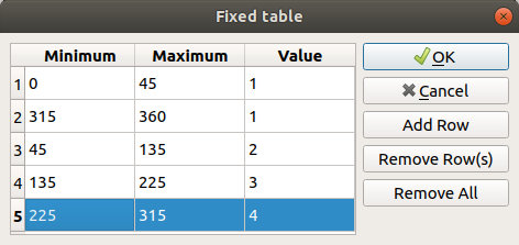
aspect 레이어로 돌아가십시오. 이제 이 레이어가 0에서 360 사이에 있는 숫자 값들을 가지고 있다는 사실을 알고 있습니다. 우리가 하고자 하는 작업은 이 레이어를 경사 방향에 따라 다른 개별 값들로 (1에서 4까지의 숫자로) 재범주화(reclassify) 하는 것입니다:
1 = 북향 (0에서 45 그리고 315에서 360까지)
2 = 동향 (45에서 135까지)
3 = 남향 (135에서 225까지)
4 = 서향 (225에서 315까지)
래스터 계산기를 통해 이 연산을 할 수도 있지만, 공식이 아주 아주 커질 겁니다.
이를 대체할 수 있는 도구가 Processing Toolbox 의 메뉴에 있는 Reclassify by table 도구입니다.
도구를 여십시오.
Choose
aspectas the Raster layerReclassification table 의 … 버튼을 클릭하십시오. 테이블 모양의 대화창이 열리고 각 범주에 대한 최소값, 최대값 및 새 값들을 선택할 수 있습니다.
Add row 버튼을 클릭하고 행 5개를 추가하십시오. 각 행을 다음 그림과 같이 채운 다음 OK 를 클릭하십시오:
각 범주의 한계값을 처리하기 위해 이 알고리즘이 사용한 메소드는 Range boundaries 가 정의합니다.
exercise_data/raster_analysis/폴더에 이 레이어를reclassified.tif로 저장하십시오.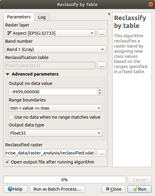
Run 을 클릭하십시오.
If you compare the native aspect layer with the
reclassified one, there are not big differences.
But by looking at the legend, you can see that the values go from
1 to 4.
이 레이어에 좀 더 나은 스타일을 적용해봅시다.
Layer Styling 패널을 여십시오.
Singleband gray 대신 Paletted/Unique values 를 선택하십시오.
Classify 버튼을 클릭하면 자동으로 값들을 가져와서 랜덤한 색상을 할당합니다:
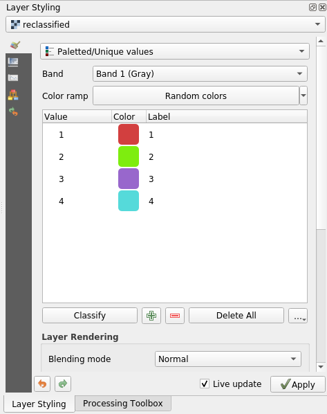
산출물이 다음처럼 보일 것입니다(색상이 랜덤하게 생성되기 때문에 다른 색상을 보게 될 수도 있습니다):
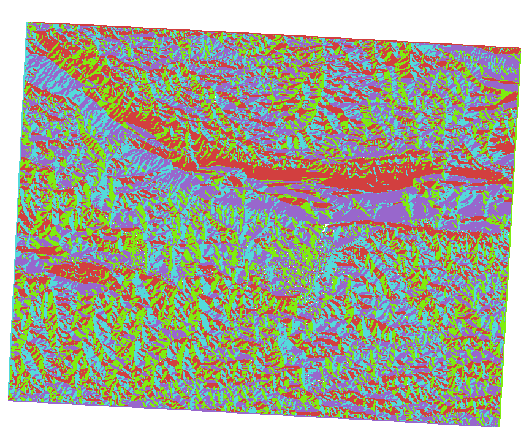
이 재범주화 작업과 레이어에 적용된 색상표 스타일 덕분에, 각각의 경사 방향 지역을 즉시 구분할 수 있습니다.
7.3.11. ★☆☆ 따라해보세요: 래스터를 쿼리하기
벡터 레이어와는 달리, 래스터 레이어는 속성 테이블을 가지고 있지 않습니다. 각 픽셀이 (래스터가 단일 밴드인지 또는 다중 밴드인지에 따라) 하나 이상의 숫자 값을 담고 있을 뿐입니다.
이번 예제에서 우리가 사용했던 모든 래스터 레이어는 밴드 하나만으로 구성돼 있습니다. 픽셀 값은 레이어에 따라 표고, 경사 방향, 또는 경사 값을 표현할 수도 있습니다.
픽셀 하나의 값을 얻으려면 래스터 레이어를 어떻게 쿼리하면 될까요?  Identify Features 버튼을 사용하면 됩니다!
속성 툴바에서 이 도구를 선택하십시오.
Click on a random location of the
srtm_41_19layer. Identify Results will appear with the value of the band at the clicked location: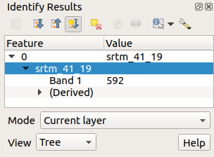
Identify Results 패널 최하단에 있는 View 메뉴에서 Table 을 선택하면 식별 결과를 현재의
tree모드에서table모드로 변경할 수 있습니다: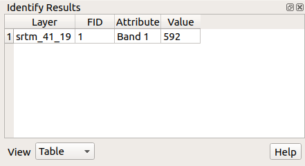
래스터의 값을 얻기 위해 픽셀 하나하나를 클릭하는 것은 좀 짜증이 날 수도 있습니다. 이 문제를 해결할 수 있는 값 도구(Value Tool) 플러그인이 존재합니다.
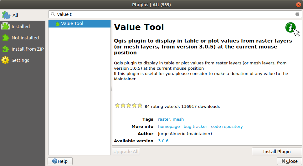
메뉴에서 항목을 클릭하십시오.
All 탭에 있는 검색란에
value t라고 입력하십시오.Value Tool 플러그인을 선택하고, Install Plugin 버튼을 누른 다음 Close 를 눌러 대화창을 닫으십시오.
새로운 Value Tool 패널이 나타날 것입니다.
팁
이 패널을 닫았다면, 메뉴 항목을 선택해서 또는 툴바에 있는 아이콘을 클릭해서 활성화시켜 다시 열 수 있습니다.
이 플러그인을 사용하려면 그냥 Enable 체크박스를 체크한 다음 Layers 패널에서
srtm_41_19레이어가 활성화(체크)된 상태인지 확인하기만 하면 됩니다.맵 위에 마우스 커서를 가져가서 픽셀들의 값을 살펴보십시오.
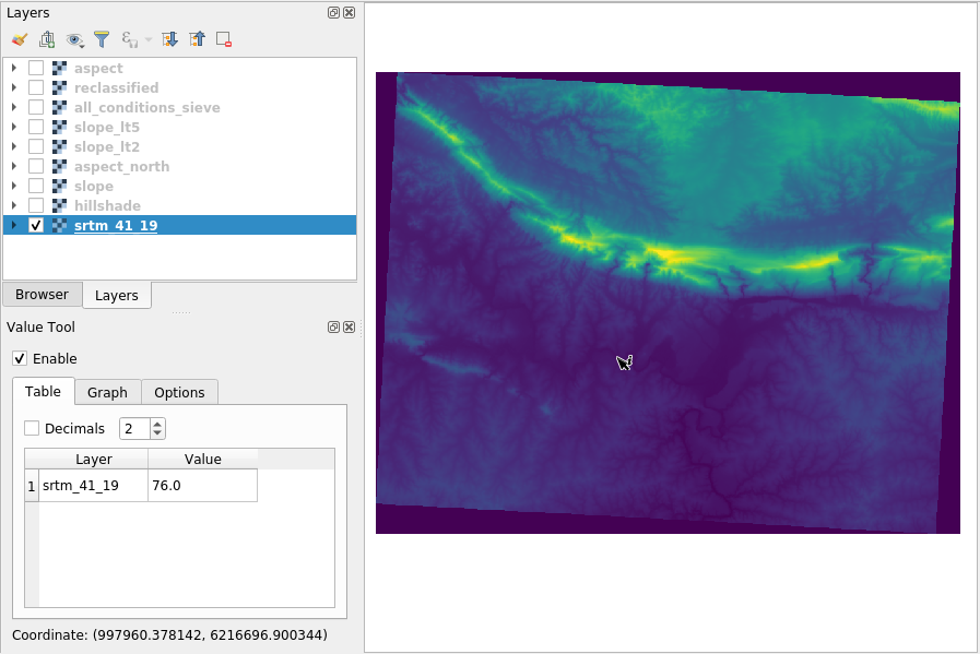
But there is more. The Value Tool plugin allows you to query all the active raster layers in the Layers panel. Set the
aspectandslopelayers active again and hover the mouse on the map: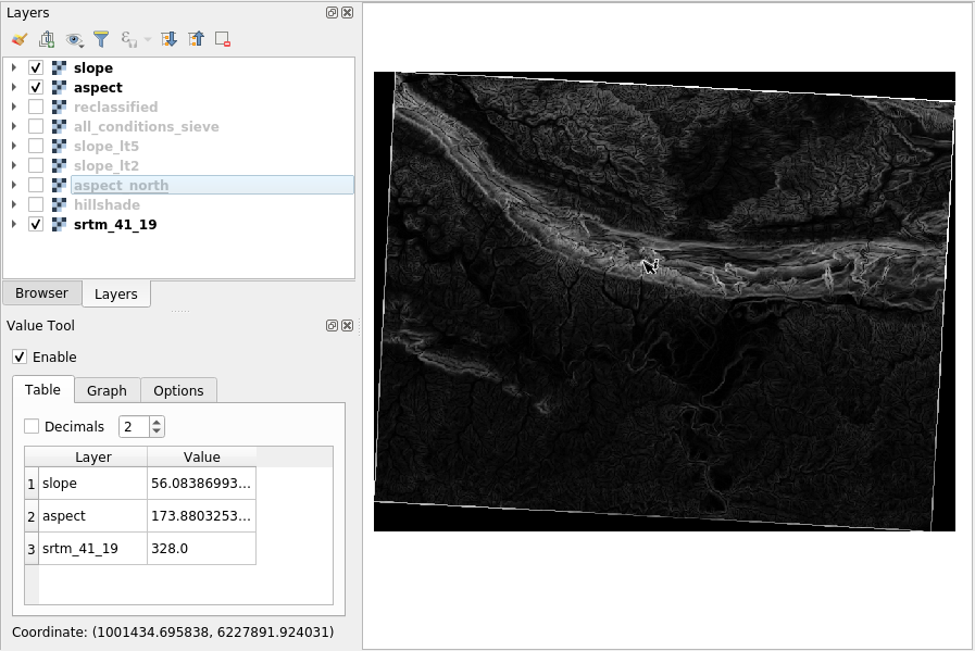
7.3.12. 결론
DEM으로부터 어떻게 모든 종류의 분석 결과를 추출할 수 있는지 배웠습니다. 이 분석 결과에는 음영기복, 경사, 그리고 경사 방향 계산이 포함됩니다. 래스터 계산기를 사용해서 이 결과들을 심도 있게 분석하고 결합하는 방법도 배웠습니다. 마지막으로, 레이어를 재범주화시키는 방법과 그 결과물을 쿼리하는 방법을 배웠습니다.
7.3.13. 다음은 무엇을 배우게 될까요?
이제 여러분은 두 가지 분석을 할 수 있습니다. 벡터 분석은 잠재적으로 적합한 계획을 보여주며, 래스터 분석은 잠재적으로 적합한 지형을 보여줍니다. 이들을 어떻게 결합해야 문제에 대한 최종 결론을 얻을 수 있을까요? 이것이 다음 강의에서 시작하는 수업의 주제입니다.