3.1. Lesson: Working with Vector Data
Vector data is arguably the most common kind of data you will find in the daily use of GIS. The vector model represents the location and shape of geographic features using points, lines and polygons (and for 3D data also surfaces and volumes), while their other properties are included as attributes (often presented as a table in QGIS). It is usually used to store discrete features, like roads and city blocks. The objects in a vector dataset are called features, and contain data that describe their location and properties.
The goal for this lesson: To learn about the structure of vector data, and how to load vector datasets into a map.
3.1.1.  Follow Along: Viewing Layer Attributes
It’s important to know that the data you will be working with does not only represent where objects are in space, but also tells you what those objects are.
From the previous exercise, you should have the rivers layer loaded in your map. The lines that you can see right now are merely the position of the rivers: this is the spatial data.
To see all the available data in the rivers layer,
select it in the Layers panel and click the  button.
It will show you a table with more data about the rivers layer. This is the layer’s Attribute table. A row is called a record, and represents a river feature. A column is called a field, and represents a property of the river. Cells show attributes.
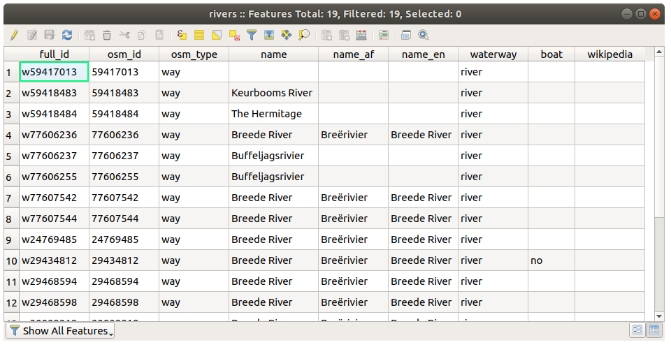
These definitions are commonly used in GIS, so it’s essential to remember them!
You may now close the attribute table.
3.1.2. Try Yourself Exploring Vector Data Attributes
How many fields are available in the rivers layer?
Tell us a bit about the
townplaces in your dataset.
3.1.3. Follow Along: Loading Vector Data From GeoPackage Database
Databases allow you to store a large volume of associated data in one file. You may already be familiar with a database management system (DBMS) such as Libreoffice Base or MS Access. GIS applications can also make use of databases. GIS-specific DBMSes (such as PostGIS) have extra functions, because they need to handle spatial data.
The GeoPackage open format is a container that
allows you to store GIS data (layers) in a single file.
Unlike the ESRI Shapefile format (e.g. the protected_areas.shp dataset
you loaded earlier), a single GeoPackage file can contain various data (both
vector and raster data) in different coordinate reference systems, as well as
tables without spatial information; all these features allow you to share data
easily and avoid file duplication.
In order to load a layer from a GeoPackage, you will first need to create the connection to it:
Click on the
 Open Data Source Manager button.
On the left click on the
 GeoPackage tab.
Click on the New button and browse to the
training_data.gpkgfile in theexercise_datafolder you downloaded before.Select the file and press Open. The file path is now added to the Geopackage connections list, and appears in the drop-down menu.
You are now ready to add any layer from this GeoPackage to QGIS.
Click on the Connect button. In the central part of the window you should now see the list of all the layers contained in the GeoPackage file.
Select the roads layer and click on the Add button.
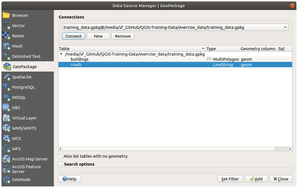
A roads layer is added to the Layers panel with features displayed on the map canvas.
Click on Close.
Congratulations! You have loaded the first layer from a GeoPackage.
3.1.4. Follow Along: Loading Vector Data From a SpatiaLite Database with the Browser
QGIS provides access to many other database formats. Like GeoPackage, the SpatiaLite database format is an extension of the SQLite library. And adding a layer from a SpatiaLite provider follows the same rules as described above: Create the connection –> Enable it –> Add the layer(s).
While this is one way to add SpatiaLite data to your map, let’s explore another powerful way to add data: the Browser.
Click the
icon to open the Data Source Manager
window.Click on the
 Browser tab.
In this tab you can see all the storage disks connected to your computer as well as entries for most of the tabs in the left. These allow quick access to connected databases or folders.
For example, click on the drop-down icon next to the
 GeoPackage entry. You’ll see the
 training-data.gpkgfile we previously connected to (and its layers, if expanded).Right-click the
 SpatiaLite entry and select
New Connection….
SpatiaLite entry and select
New Connection….Navigate to the
exercise_datafolder, select thelanduse.sqlitefile and click Open.Notice that a
 landuse.sqlite entry has
been added under the SpatiaLite one.
landuse.sqlite entry has
been added under the SpatiaLite one.Expand the
landuse.sqlite entry.Double-click the
 landuse layer or select and
drag-and-drop it onto the map canvas. A new layer is added to the
Layers panel and its features are displayed on the map canvas.
landuse layer or select and
drag-and-drop it onto the map canvas. A new layer is added to the
Layers panel and its features are displayed on the map canvas.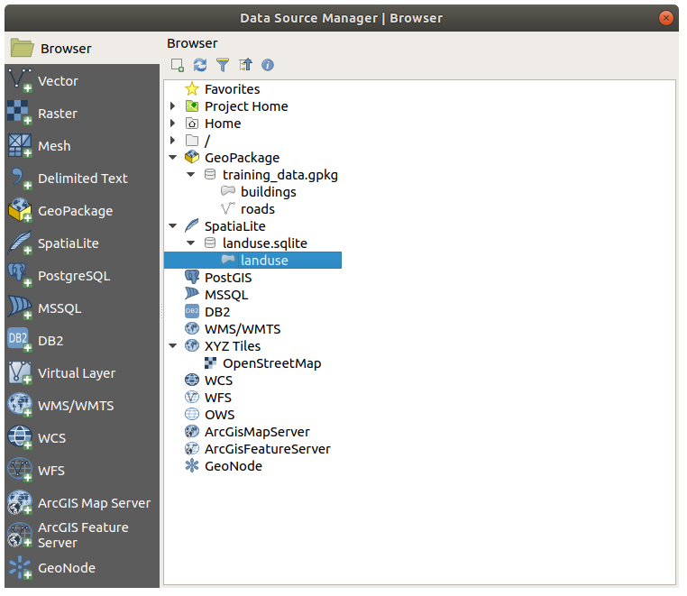
Tip
Enable the Browser panel in and use it to add your data. It’s a handy shortcut for the tab, with the same functionality.
Note
Remember to save your project frequently! The project file doesn’t contain any of the data itself, but it remembers which layers you loaded into your map.
3.1.5.  Try Yourself Load More Vector Data
Load the following datasets from the exercise_data folder into your map
using any of the methods explained above:
buildings
water
3.1.6. Follow Along: Reordering the Layers
The layers in your Layers list are drawn on the map in a certain order. The layer at the bottom of the list is drawn first, and the layer at the top is drawn last. By changing the order that they are shown on the list, you can change the order they are drawn in.
Note
You can alter this behavior using the Control rendering order checkbox beneath the Layer Order panel. We will however not discuss this feature yet.
The order in which the layers have been loaded into the map is probably not logical at this stage. It’s possible that the road layer is completely hidden because other layers are on top of it.
For example, this layer order…
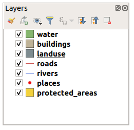
… would result in roads and places being hidden as they run underneath the polygons of the landuse layer.
To resolve this problem:
Click and drag on a layer in the Layers list.
Reorder them to look like this:
You’ll see that the map now makes more sense visually, with roads and buildings appearing above the land use regions.
3.1.7. In Conclusion
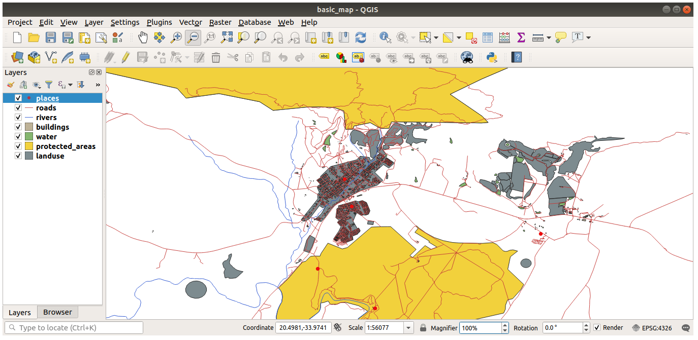
Now you’ve added all the layers you need from several different sources.
3.1.8. What’s Next?
Using the random palette automatically assigned when loading the layers, your current map is probably not easy to read. It would be preferable to assign your own choice of colors and symbols. This is what you’ll learn to do in the next lesson.