17.10. The raster calculator. No-data values
Nota
In this lesson we will see how to use the raster calculator to perform some operations on raster layers. We will also explain what are no–data values and how the calculator and other algorithms deal with them
The raster calculator is one of the most powerful algorithms that you will find. It’s a very flexible and versatile algorithm that can be used for many different calculations, and one that will soon become an important part of your toolbox.
In this lesson we will be performing some calculation with the raster calculator, most of them rather simple. This will let us see how it is used and how it deals with some particular situations that it might find. Understanding that is important to later get the expected results when using the calculator, and also to understand certain techniques that are commonly applied with it.
Open the QGIS project corresponding to this lesson and you will see that it contains several raster layers.
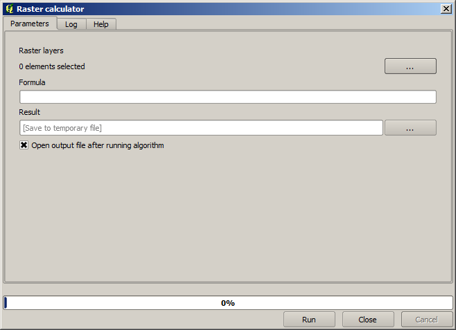
Now open the toolbox and open the dialog corresponding to the raster calculator.
Nota
The interface is different in recent versions.
The dialog contains 2 parameters.
The layers to use for the analysis. This is a multiple input, that meaning that you can select as many layers as you want. Click on the button on the right–hand side and then select the layers that you want to use in the dialog that will appear.
The formula to apply. The formula uses the layers selected in the above parameter, which are named using alphabet letters (
a, b, c...) org1, g2, g3...as variable names. That is, the formulaa + 2 * bis the same asg1 + 2 * g2and will compute the sum of the value in the first layer plus two times the value in the second layer. The ordering of the layers is the same ordering that you see in the selection dialog.
Aviso
The calculator is case sensitive.
To start with, we will change the units of the DEM from meters to feet. The formula we need is the following one:
h' = h * 3.28084
Select the DEM in the layers field and type a * 3.28084 in the formula field.
Aviso
For non English users: use always «.», not «,».
Click Run to run the algorithm. You will get a layer that has the same appearance of the input layer, but with different values. The input layer that we used has valid values in all its cells, so the last parameter has no effect at all.
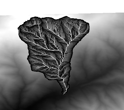
Let’s now perform another calculation, this time on the accflow layer. This layer contains values of accumulated flow, a hydrological parameter. It contains those values only within the area of a given watershed, with no–data values outside of it. As you can see, the rendering is not very informative, due to the way values are distributed. Using the logarithm of that flow accumulation will yield a much more informative representation. We can calculate that using the raster calculator.
Open the algorithm dialog again, select the accflow layer as the only input layer, and enter the following formula: log(a).
Here is the layer that you will get.
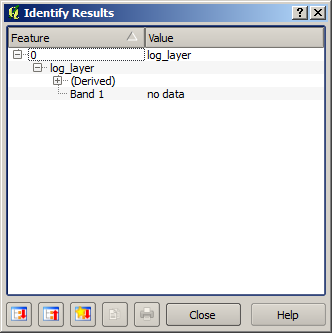
If you select the Identify tool to know the value of a layer at a given point, select the layer that we have just created, and click on a point outside of the basin, you will see that it contains a no–data value.
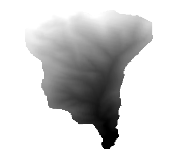
For the next exercise we are going to use two layers instead of one, and we are going to get a DEM with valid elevation values only within the basin defined in the second layer. Open the calculator dialog and select both layers of the project in the input layers field. Enter the following formula in the corresponding field:
a/a * b
a refers to the accumulated flow layer (since it is the first one to appear in the list) and b refers to the DEM. What we are doing in the first part of the formula here is to divide the accumulated flow layer by itself, which will result in a value of 1 inside the basin, and a no–data value outside. Then we multiply by the DEM, to get the elevation value in those cells inside the basin (DEM * 1 = DEM) and the no–data value outside (DEM * no_data = no_data)
Here is the resulting layer.
This technique is used frequently to mask values in a raster layer, and is useful whenever you want to perform calculations for a region other that the arbitrary rectangular region that is used by raster layer. For instance, an elevation histogram of a raster layer doesn’t have much meaning. If it is instead computed using only values corresponding to a basin (as in he case above), the result that we obtain is a meaningful one that actually gives information about the configuration of the basin.
There are other interesting things about this algorithm that we have just run, apart from the no–data values and how they are handled. If you have a look at the extents of the layers that we have multiplied (you can do it double–clicking on their names of the layer in the table of contents and looking at their properties), you will see that they are not the same, since the extent covered by the flow accumulation layer is smaller that the extent of the full DEM.
That means that those layers do not match, and that they cannot be multiplied directly without homogenizing those sizes and extents by resampling one or both layers. However, we did not do anything. QGIS takes care of this situation and automatically resamples input layers when needed. The output extent is the minimum covering extent calculated from the input layers, and the minimum cell size of their cellsizes.
In this case (and in most cases), this produces the desired results, but you should always be aware of the additional operations that are taking place, since they might affect the result. In cases when this behaviour might not be the desired, manual resampling should be applied in advance. In later chapters, we will see more about the behaviour of algorithms when using multiple raster layers.
Let’s finish this lesson with another masking exercise. We are going to calculate the slope in all areas with an elevation between 1000 and 1500 meters.
In this case, we do not have a layer to use as a mask, but we can create it using the calculator.
Run the calculator using the DEM as only input layer and the following formula
ifelse(abs(a-1250) < 250, 1, 0/0)
As you can see, we can use the calculator not only to do simple algebraic operations, but also to run more complex calculation involving conditional sentences, like the one above.
The result has a value of 1 inside the range we want to work with, and no-data in cells outside of it.
The no-data value comes from the 0/0 expression. Since that is an undetermined value, SAGA will add a NaN (Not a Number) value, which is actually handled as a no-data value. With this little trick you can set a no-data value without needing to know what the no–data value of the cell is.
Now you just have to multiply it by the slope layer included in the project, and you will get the desired result.
All that can be done in a single operation with the calculator. We leave that as an exercise for the reader.