6.2. Lesson: Vector Analysis
Vector data can also be analyzed to reveal how different features interact with each other in space. There are many different analysis-related functions, so we won’t go through them all. Rather, we will pose a question and try to solve it using the tools that QGIS provides.
The goal for this lesson: To ask a question and solve it using analysis tools.
6.2.1. ★☆☆ The GIS Process
Before we start, it would be useful to give a brief overview of a process that can be used to solve a problem. The way to go about it is:
State the Problem
Get the Data
Analyze the Problem
Present the Results
6.2.2. ★☆☆ The Problem
Let’s start off the process by deciding on a problem to solve. For example, you are an estate agent and you are looking for a residential property in Swellendam for clients who have the following criteria:
It needs to be in Swellendam
It must be within reasonable driving distance of a school (say 1km)
It must be more than 100m squared in size
Closer than 50m to a main road
Closer than 500m to a restaurant
6.2.3. ★☆☆ The Data
To answer these questions, we are going to need the following data:
The residential properties (buildings) in the area
The roads in and around the town
The location of schools and restaurants
The size of buildings
These data are available through OSM, and you should find that the dataset you have been using throughout this manual also can be used for this lesson.
If you want to download data from another area, jump to the Introduction Chapter to read how to do it.
Note
Although OSM downloads have consistent data fields, the coverage and detail does vary. If you find that your chosen region does not contain information on restaurants, for example, you may need to chose a different region.
6.2.4. ★☆☆ Follow Along: Start a Project and get the Data
We first need to load the data to work with.
Start a new QGIS project
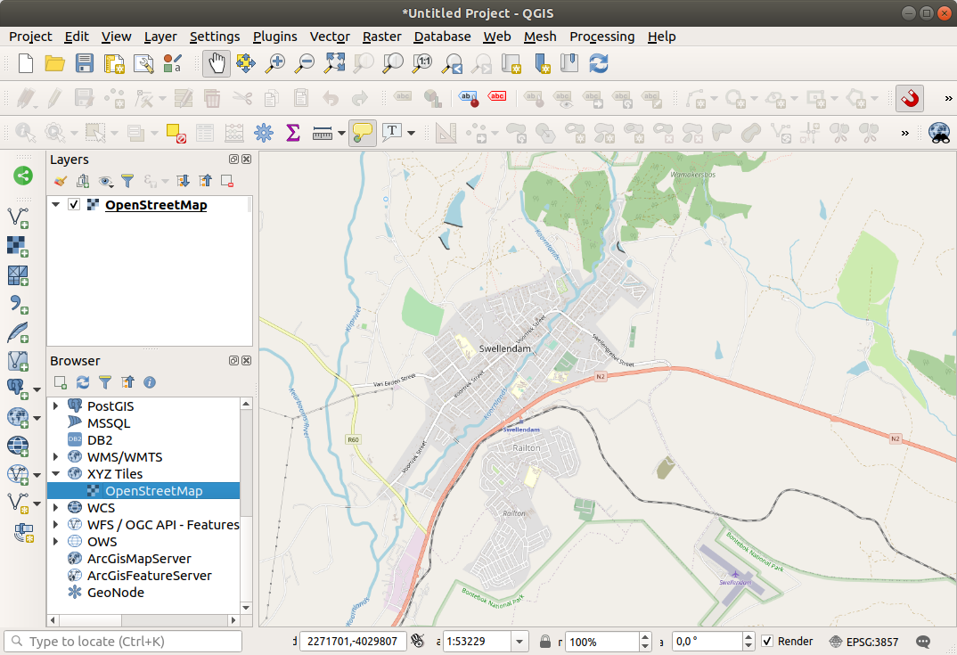
If you want, you can add a background map. Open the Browser and load the OSM background map from the XYZ Tiles menu.
In the
training_data.gpkgGeopackage database, you will find most the datasets we will use in this chapter:buildingsroadsrestaurantsschools
Load them, and also
landuse.sqlite.Zoom to the layer extent to see Swellendam, South Africa
Before proceeding we will filter the
roadslayer, in order to have only some specific road types to work with.Some roads in OSM datasets are listed as
unclassified,tracks,pathandfootway. We want to exclude these from our dataset and focus on the other road types, more suitable for this exercise.Moreover, OSM data might not be updated everywhere, and we will also exclude
NULLvalues.Right click on the
roadslayer and choose Filter….In the dialog that pops up we filter these features with the following expression:
"highway" NOT IN ('footway', 'path', 'unclassified', 'track') AND "highway" IS NOT NULL
The concatenation of the two operators
NOTandINexcludes all the features that have these attribute values in thehighwayfield.IS NOT NULLcombined with theANDoperator excludes roads with no value in thehighwayfield.Note the
 icon next to the
 roadslayer. It helps you remember that this layer has a filter activated, so some features may not be available in the project.
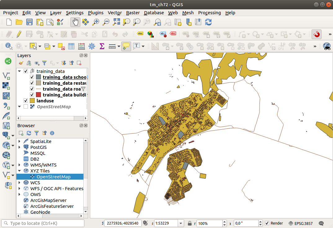
The map with all the data should look like the following one:
6.2.5. ★☆☆ Try Yourself: Convert Layers’ CRS
Because we are going to be measuring distances within our layers, we need to change the layers’ CRS. To do this, we need to select each layer in turn, save the layer to a new one with our new projection, then import that new layer into our map.
You have many different options, e.g. you can export each layer as an
ESRI Shapefile format dataset, you can append the layers to an
existing GeoPackage file, or you can create another GeoPackage file
and fill it with the new reprojected layers.
We will show the last option, so the training_data.gpkg will
remain clean.
Feel free to choose the best workflow for yourself.
Note
In this example, we are using the WGS 84 / UTM zone 34S CRS, but you should use a UTM CRS which is more appropriate for your region.
Right click the
roadslayer in the Layers panelClick Export –> Save Features As…
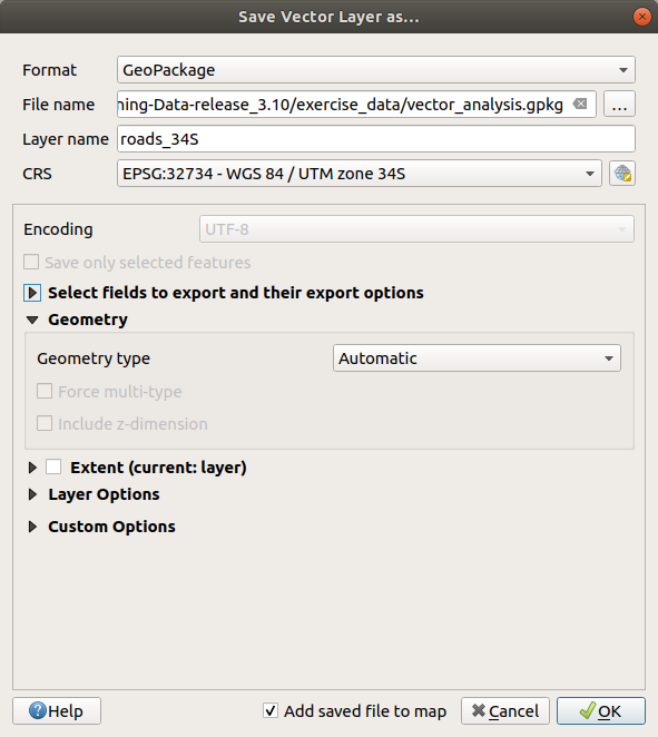
In the Save Vector Layer As dialog choose GeoPackage as Format
Click on … for the File name, and name the new GeoPackage
vector_analysisChange the Layer name to
roads_34SChange the CRS to WGS 84 / UTM zone 34S
Click on OK:
This will create the new GeoPackage database and add the
roads_34Slayer.Repeat this process for each layer, creating a new layer in the
vector_analysis.gpkgGeoPackage file with_34Sappended to the original name.On macOS, press the Replace button in the dialog that pops up to allow QGIS to overwrite the existing GeoPackage.
Note
When you choose to save a layer to an existing GeoPackage, QGIS will add that layer next to the existing layers in the GeoPackage, if no layer of the same name already exists.
Remove each of the old layers from the project
Once you have completed the process for all the layers, right click on any layer and click Zoom to layer extent to focus the map to the area of interest.
Now that we have converted OSM data to a UTM projection, we can begin our calculations.
6.2.6. ★☆☆ Follow Along: Analyzing the Problem: Distances From Schools and Roads
QGIS allows you to calculate distances between any vector object.
Make sure that only the
roads_34Sandbuildings_34Slayers are visible (to simplify the map while you’re working)Click on the to open the analytical core of QGIS. Basically, all algorithms (for vector and raster analysis) are available in this toolbox.
We start by calculating the area around the
roads_34Sby using the Buffer algorithm. You can find it in the group.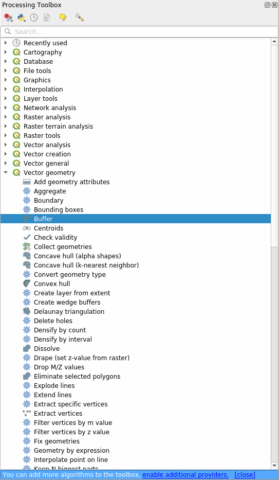
Or you can type
bufferin the search menu in the upper part of the toolbox: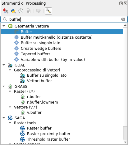
Double click on it to open the algorithm dialog
Select
roads_34Sas Input layer, set Distance to 50 and use the default values for the rest of the parameters.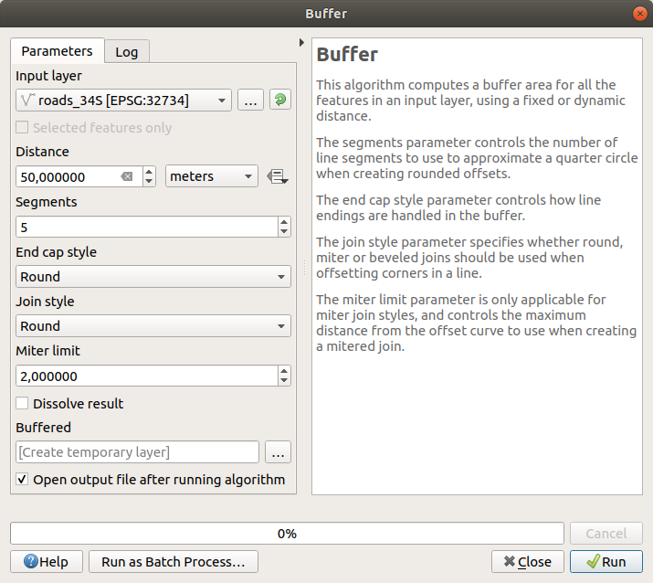
The default Distance is in meters because our input dataset is in a Projected Coordinate System that uses meter as its basic measurement unit. You can use the combo box to choose other projected units like kilometers, yards, etc.
Note
If you are trying to make a buffer on a layer with a Geographical Coordinate System, Processing will warn you and suggest to reproject the layer to a metric Coordinate System.
By default, Processing creates temporary layers and adds them to the Layers panel. You can also append the result to the GeoPackage database by:
Clicking on the … button and choose Save to GeoPackage…
Naming the new layer
roads_buffer_50mSaving it in the
vector_analysis.gpkgfile
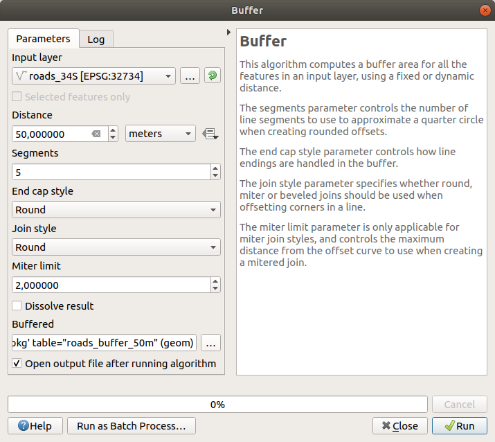
Click on Run, and then close the Buffer dialog
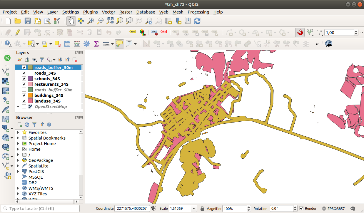
Now your map will look something like this:
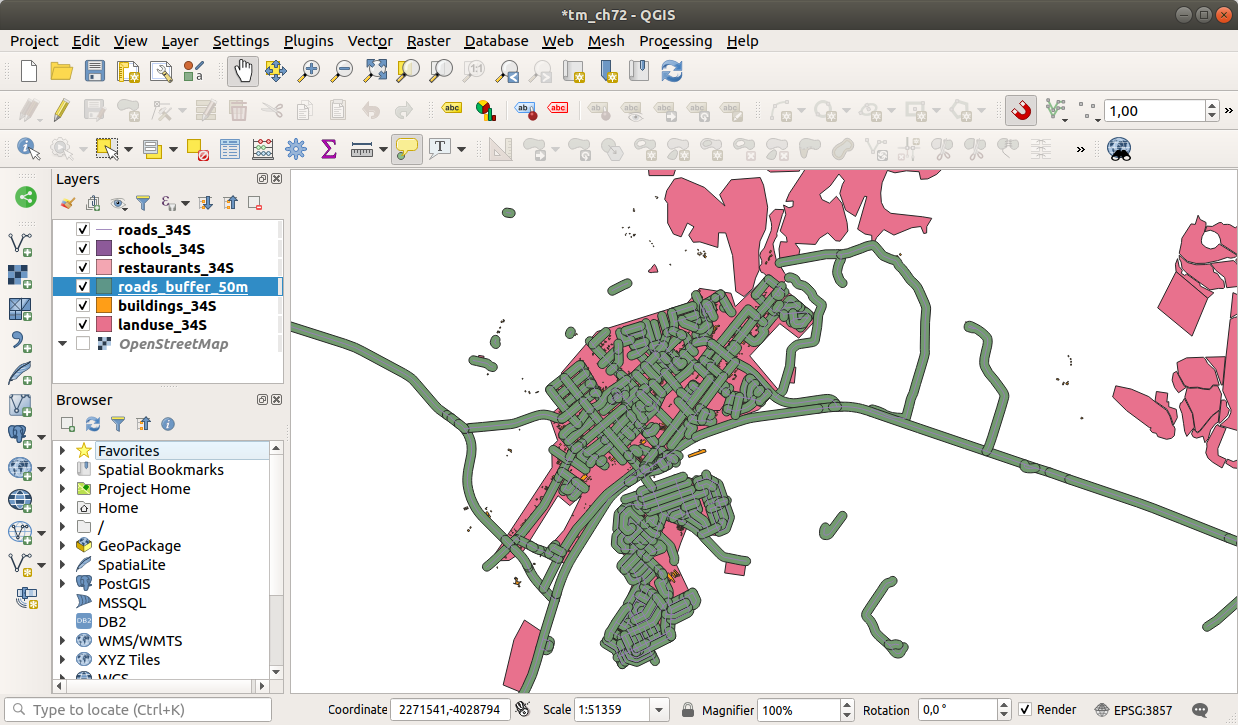
If your new layer is at the top of the Layers list, it will probably obscure much of your map, but this gives you all the areas in your region which are within 50m of a road.
Notice that there are distinct areas within your buffer, which correspond to each individual road. To get rid of this problem:
Uncheck the
roads_buffer_50mlayer and re-create the buffer with Dissolve results enabled.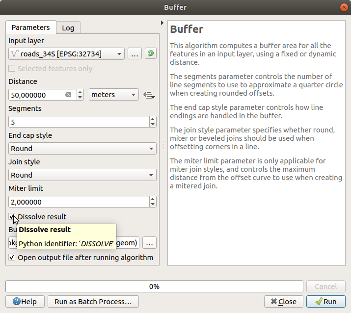
Save the output as
roads_buffer_50m_dissolvedClick Run and close the Buffer dialog
Once you have added the layer to the Layers panel, it will look like this:
Now there are no unnecessary subdivisions.
Note
The Short Help on the right side of the dialog explains how the algorithm works. If you need more information, just click on the Help button in the bottom part to open a more detailed guide of the algorithm.
6.2.7. ★☆☆ Try Yourself: Distance from schools
Use the same approach as above and create a buffer for your schools.
It shall be 1 km in radius.
Save the new layer in the vector_analysis.gpkg file as schools_buffer_1km_dissolved.
Answer
Your buffer dialog should look like this:
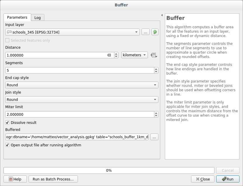
The Buffer distance is 1 kilometer.
The Segments to approximate value is set to
20. This is optional, but it’s recommended, because it makes the output buffers look smoother. Compare this: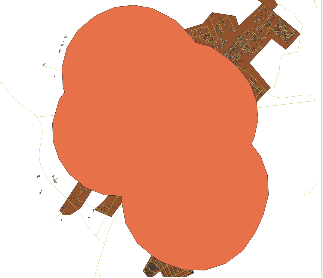
To this:
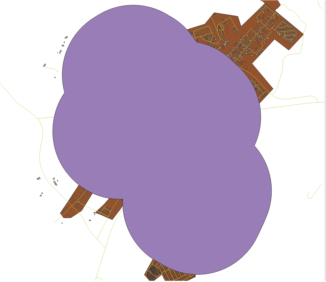
The first image shows the buffer with the Segments to approximate
value set to 5 and the second shows the value set to 20.
In our example, the difference is subtle, but you can see that the buffer’s edges
are smoother with the higher value.
6.2.8. ★☆☆ Follow Along: Overlapping Areas
Now we have identified areas where the road is less than 50 meters away and areas where there is a school within 1 km (direct line, not by road). But obviously, we only want the areas where both of these criteria are satisfied. To do that, we will need to use the Intersect tool. You can find it in group in the Processing Toolbox.
Use the two buffer layers as Input layer and Overlay layer, choose
vector_analysis.gpkgGeoPackage in Intersection with Layer nameroad_school_buffers_intersect. Leave the rest as suggested (default).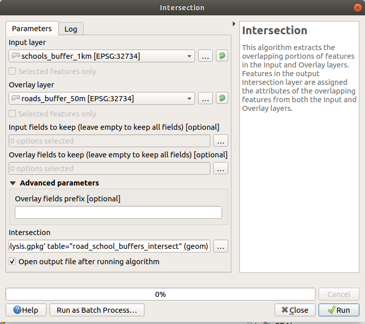
Click Run.
In the image below, the blue areas are where both of the distance criteria are satisfied.
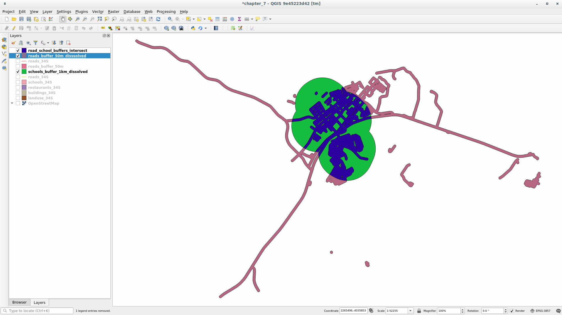
You may remove the two buffer layers and only keep the one that shows where they overlap, since that’s what we really wanted to know in the first place:
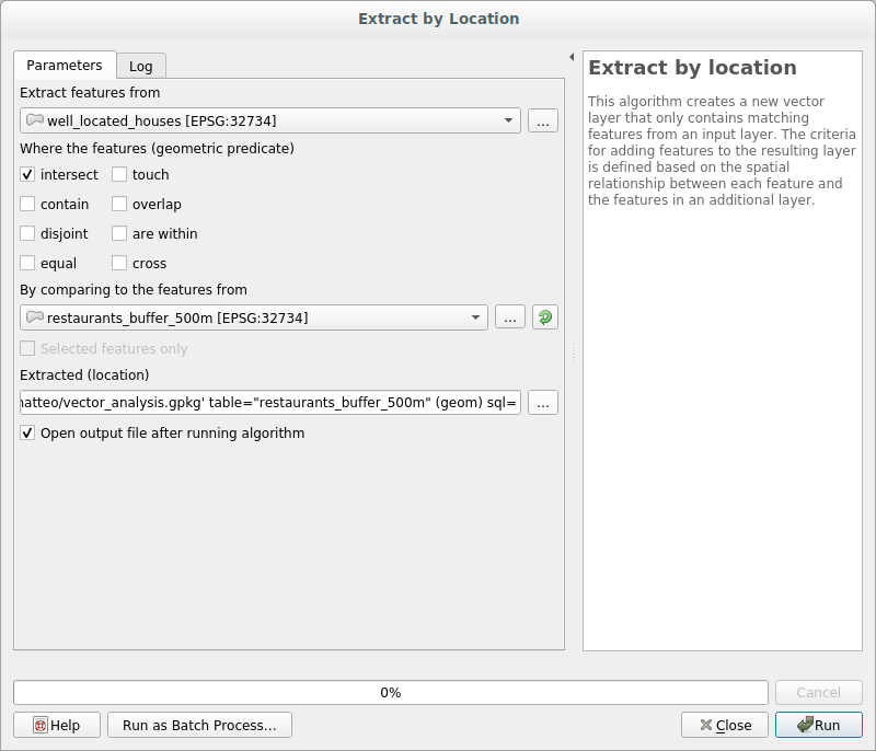
6.2.9. ★☆☆ Follow Along: Extract the Buildings
Now you’ve got the area that the buildings must overlap. Next, you want to extract the buildings in that area.
Look for the menu entry within the Processing Toolbox
Select
buildings_34Sin Extract features from. Check intersect in Where the features (geometric predicate), select the buffer intersection layer in By comparing to the features from. Save to thevector_analysis.gpkg, and name the layerwell_located_houses.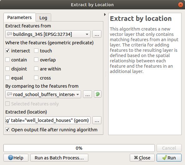
Click Run and close the dialog
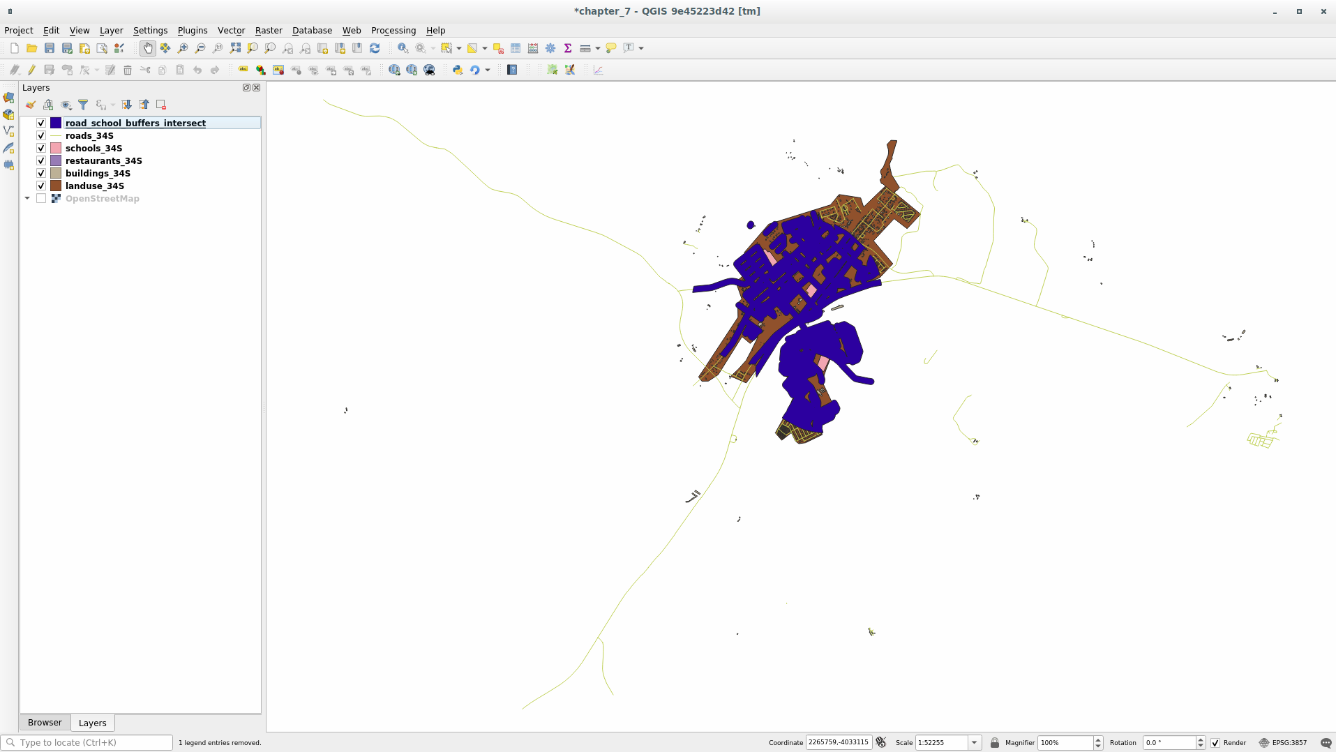
You will probably find that not much seems to have changed. If so, move the
well_located_houseslayer to the top of the layers list, then zoom in.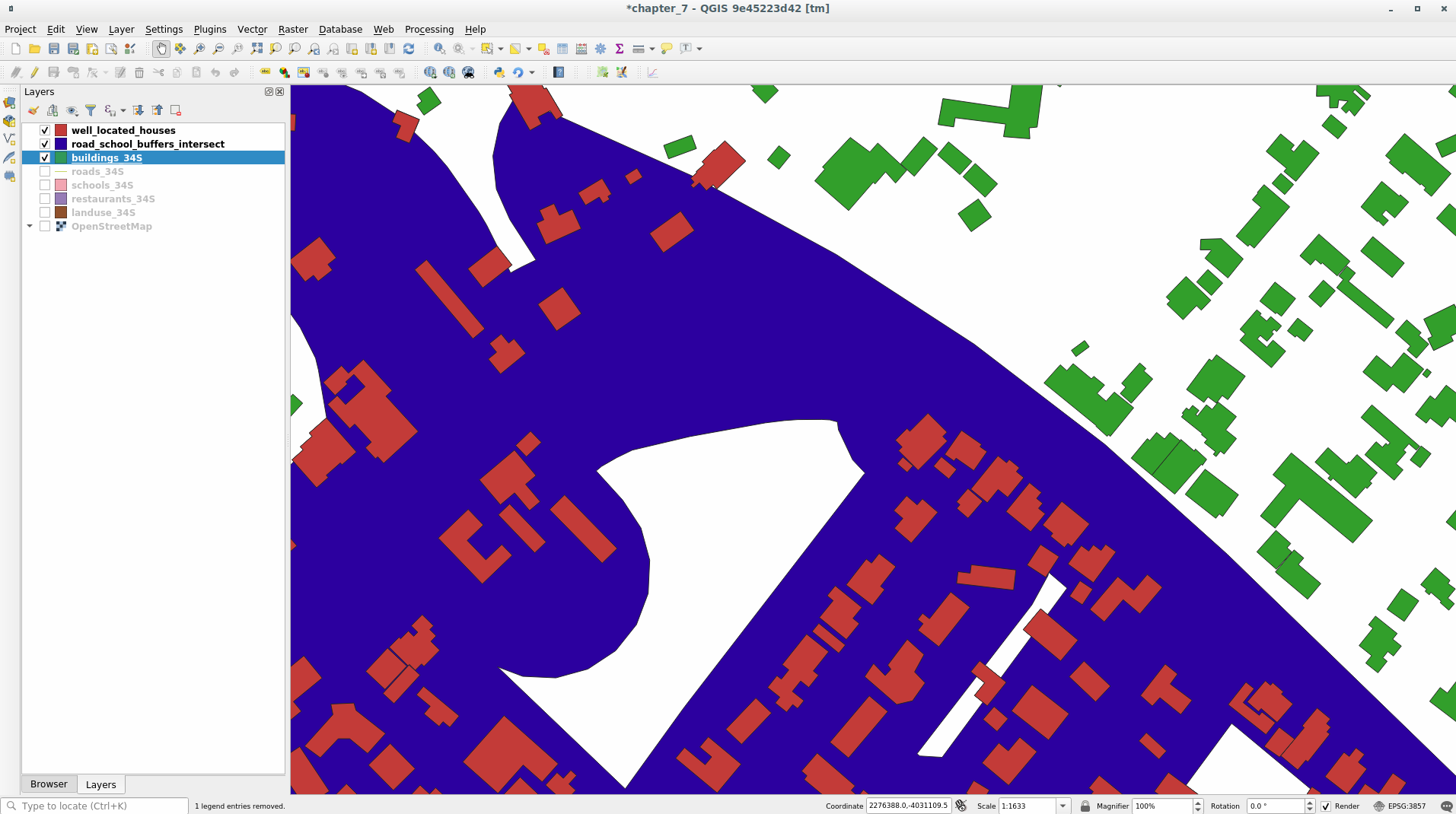
The red buildings are those which match our criteria, while the buildings in green are those which do not.
Now you have two separated layers and can remove
buildings_34Sfrom the layer list.
6.2.10. ★★☆ Try Yourself: Further Filter our Buildings
We now have a layer which shows us all the buildings within 1km of a school and within 50m of a road. We now need to reduce that selection to only show buildings which are within 500m of a restaurant.
Using the processes described above, create a new layer called
houses_restaurants_500m which further filters your
well_located_houses layer to show only those which are
within 500m of a restaurant.
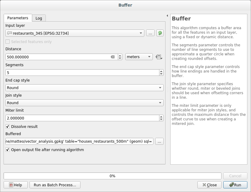
Answer
To create the new houses_restaurants_500m layer, we go through a two step
process:
First, create a buffer of 500m around the restaurants and add the layer to the map:
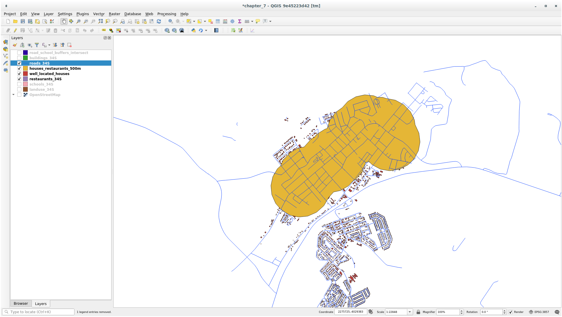
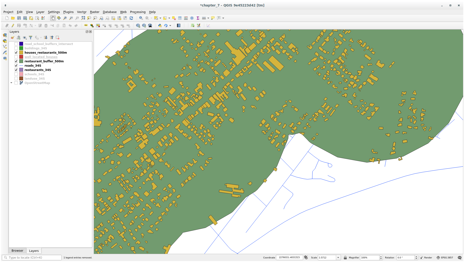
Next, extract buildings within that buffer area:
Your map should now show only those buildings which are within 50m of a road, 1km of a school and 500m of a restaurant:
6.2.11. ★☆☆ Follow Along: Select Buildings of the Right Size
To see which buildings are of the correct size (more than 100 square meters), we need to calculate their size.
Select the
houses_restaurants_500mlayer and open the Field Calculator by clicking on the Open Field Calculator button in the main toolbar or in
the attribute table window
Open Field Calculator button in the main toolbar or in
the attribute table windowSelect Create a new field, set the Output field name to
AREA, choose Decimal number (real) as Output field type, and choose$areafrom the group.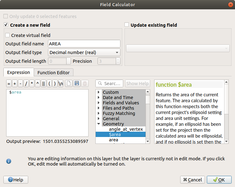
The new field
AREAwill contain the area of each building in square meters.Click OK. The
AREAfield has been added at the end of the attribute table.Click the
 Toggle Editing button to finish
editing, and save your edits when prompted.
Toggle Editing button to finish
editing, and save your edits when prompted.In the tab of the layer properties, set the Provider Feature Filter to
"AREA >= 100.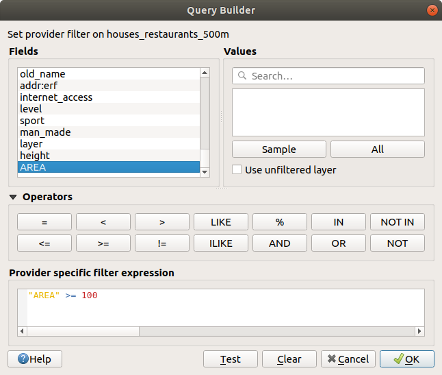
Click OK.
Your map should now only show you those buildings which match our starting criteria and which are more than 100 square meters in size.
6.2.12. ★☆☆ Try Yourself:
Save your solution as a new layer, using the approach you learned
above for doing so.
The file should be saved within the same GeoPackage database, with
the name solution.
6.2.13. In Conclusion
Using the GIS problem solving approach together with QGIS vector analysis tools, you were able to solve a problem with multiple criteria quickly and easily.
6.2.14. What’s Next?
In the next lesson, we will look at how to calculate the shortest distance along roads from one point to another.