Важно
Перевод - это работа сообщества : ссылка:Вы можете присоединиться. Эта страница в настоящее время переводится |прогресс перевода|.
6.2. Lesson: Vector Analysis
Векторные данные также можно анализировать, чтобы узнать, как различные объекты взаимодействуют друг с другом в пространстве. Есть множество различных функций, связанных с анализом, но мы не будем их все рассматривать. Мы лучше зададим вопрос и попытаемся найти на него ответ с помощью инструментов QGIS.
Цель этого урока: Задать вопрос и решить его с помощью инструментов анализа.
6.2.1. ★☆☆ The GIS Process
Перед тем как начать было бы хорошо сделать краткий обзор процесса, который надо пройти для решения проблемы. Он представлен ниже:
Обозначить проблему.
Получить данные.
Проанализировать проблему.
Представить результаты.
6.2.2. ★☆☆ The Problem
Начнем с определения проблемы, которую нужно решить. Например, вы являетесь агентом по продаже недвижимости и ищете жилое помещение в Свеллендаме / Swellendam для своих клиентов со следующими критериями:
Жилое помещение должно находиться в Swellendam.
Оно должно находиться в пределах умеренного расстояния от школы (например, 1 км).
Его площадь должна быть более 100 квадратных метров.
Находиться на расстоянии менее чем 50 метров от главной дороги.
Находиться на расстоянии менее чем 500 метров от какого-нибудь ресторана.
6.2.3. ★☆☆ The Data
Чтобы ответить на эти вопросы, нам нужны следующие данные:
Жилые помещения (здания) в этом районе.
Дороги внутри города и вокруг него.
Месторасположение школ и ресторанов.
Размер зданий.
Эти данные можно получить через OSM (OpenStreetMap) и вы узнаете, что набор данных, который вы использовали в этом руководстве, также можно использовать для выполнения этого урока.
Если вы хотите загрузить данные из другой местности, перейдите в Раздел Введение и ознакомьтесь, как это можно сделать.
Примечание
Хотя загружаемые файлы OSM содержат согласованные поля данных, охват и детализация могут быть разными. Если вы обнаружили, что выбранный вами регион, к примеру, не содержит сведения по ресторанам, то вам, возможно, надо выбрать другой регион.
6.2.4. ★☆☆ Follow Along: Start a Project and get the Data
Сначала нам надо загрузить данные, с которыми мы будет работать.
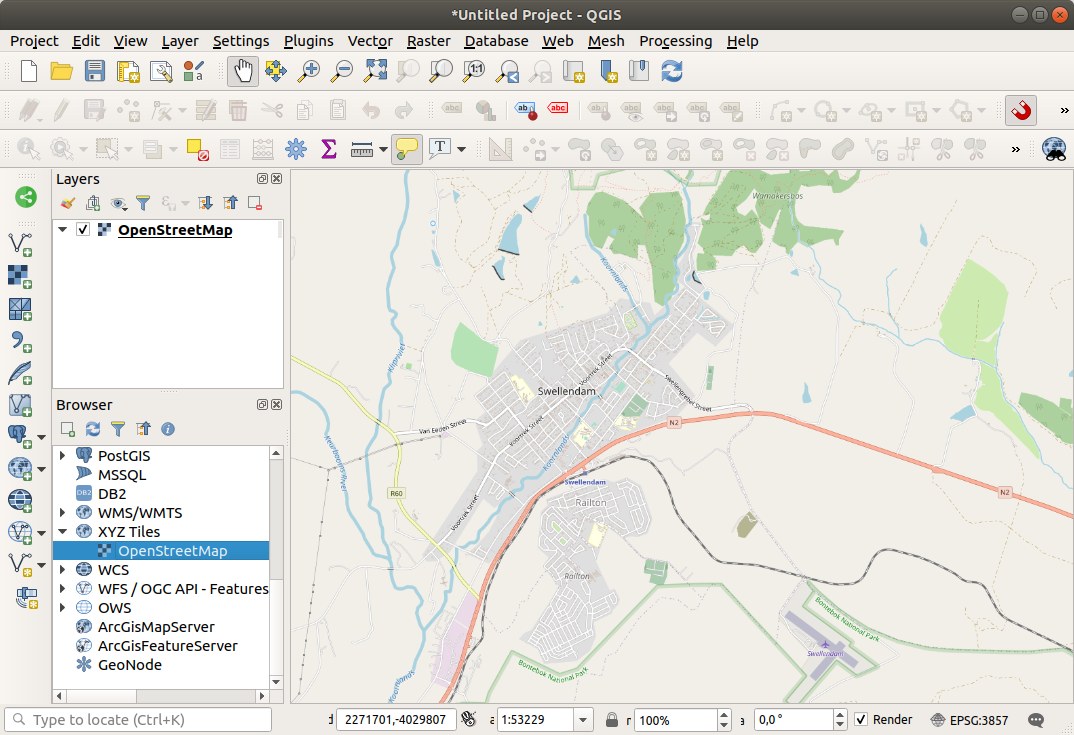
Начать новый проект QGIS.
Если хотите, можете добавить фоновую карту. Откройте Browser и загрузите фоновую карту OSM из меню XYZ Tiles.
В базе данных Geopackage
training_data.gpkgвы сможете найти большинство наборов данных, которые мы будем использовать в это разделе:buildingsroadsrestaurantsschools
Загрузите их, а также
landuse.sqlite.Увеличьте масштаб слоя, чтобы увидеть Свеллендам в Южной Африке.
Before proceeding we will filter the
roadslayer, in order to have only some specific road types to work with.Некоторые дороги в наборах данных OSM перечислены как
unclassified,tracks,path, а такжеfootway. Нам надо исключить их из нашего набора данных и сосредоточиться на других типах дорог, которые больше подходят для этого упражнения.Кроме того, не все данные OSM могут быть актуализированы и мы также надо исключить значения
NULL.Кликните правой кнопкой мыши на слой
roadsи выберите Filter….В диалоговом окне, которое появится, мы должны отфильтровать эти объекты с помощью следующего выражения:
"highway" NOT IN ('footway', 'path', 'unclassified', 'track') AND "highway" IS NOT NULL
Объединение двух команд
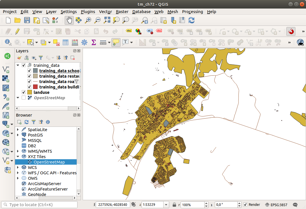
NOTиINисключает все объекты, которые имеют эти атрибуты значений в полеhighway.IS NOT NULLв сочетании сANDисключает дороги, не имеющие значения в полеhighway.Note the
 icon next to the
 roadslayer. It helps you remember that this layer has a filter activated, so some features may not be available in the project.
Карта со всеми данными должна выглядеть следующим образом:
6.2.5. ★☆☆ Try Yourself: Convert Layers“ CRS
Так как мы собираемся измерить расстояния внутри наших слоев, нам надо изменить ССК слоев. Для этого нам надо выбрать каждый слой по очереди, сохранить слой по-новому с нашей новой проекцией, а затем импортировать этот новый слой на нашу карту.
У вас появится много различных опций, например, вы сможете экспортировать каждый слой как набор данных формата ESRI Shapefile, вы можете добавить слои в существующий файл GeoPackage или создать другой файл GeoPackage и заполнить его новыми пере-проецированными слоями. Мы покажем последнюю опцию, чтобы training_data.gpkg остался чистым. Вы сможете выбрать для себя свой лучший рабочий процесс.
Примечание
На этом примере мы используем ССК WGS 84 / UTM zone 34S, но вы должны использовать UTM ССК, который больше подходит для вашего региона.
Right click the
roadslayer in the Layers panelКликните Export –> Save Features As…
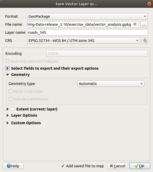
В диалоговом окне Save Vector Layer As выберите GeoPackage в качестве Format.
Кликните на … для File name и назовите новый GeoPackage
vector_analysis.Изменить Layer name на
roads_34S.Измените CRS на WGS 84 / UTM зону 34S.
Кликните на OK:
Это позволит создать новую базу данных GeoPackage и добавить слой
roads_34S.Repeat this process for each layer, creating a new layer in the
vector_analysis.gpkgGeoPackage file with_34Sappended to the original name.On macOS, press the Replace button in the dialog that pops up to allow QGIS to overwrite the existing GeoPackage.
Примечание
When you choose to save a layer to an existing GeoPackage, QGIS will add that layer next to the existing layers in the GeoPackage, if no layer of the same name already exists.
Remove each of the old layers from the project
После того, как вы завершили процесс по всем слоям, вам надо кликнуть правой кнопкой мыши на любой слой и нажать Zoom to layer extent, чтобы сфокусировать карту на местность, которая вас интересует.
Теперь, когда мы преобразовали данные OSM в Универсальную поперечную проекцию Меркатора (УППМ), мы можем начать наши вычисления.
6.2.6. ★☆☆ Follow Along: Analyzing the Problem: Distances From Schools and Roads
QGIS позволяет рассчитывать расстояния между любыми векторными объектами.
Удостоверьтесь в том, что только слои
roads_34Sиbuildings_34Sбыли видны (для упрощения карты во время работы).Кликни на для того, чтобы открыть аналитическое ядро QGIS. В основном, в этом наборе инструментов имеются все алгоритмы (для векторного и растрового анализа).
Мы можем начать рассчитывать площади вокруг
roads_34Sиспользуя алгоритм Buffer. Вы можете найти его в группе .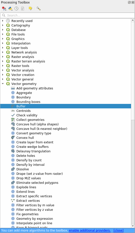
Или вы можете набрать в меню поиска
bufferв верхней части панели инструментов: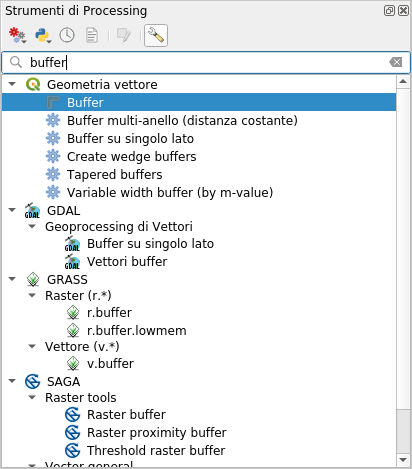
Два раза кликните по нему, чтобы открыть диалоговое окно алгоритма.
Выбираете
roads_34Sв качестве Input layer, указываете Distance до 50 и используйте значения по умолчанию для остальных параметров.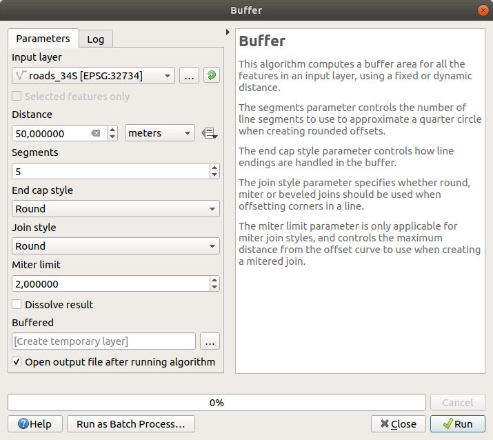
По умолчанию Distance измеряется в метрах, потому что наш входной набор данных находится в системе координат проекции, которая использует метр в качестве основной единицы измерения. Вы можете использовать поле со списком, чтобы выбрать другие проецируемые единицы, такие как километры, ярды и т.д.
Примечание
Если вы пытаетесь создать буфер на слое с географической системой координат, система при обработке предупредит вас и предложит перепроецировать слой в метрическую систему координат.
По умолчанию при обработке создаются временные слои и они добавляется в панель Layers. Вы также можете приложить результат в базу данных GeoPackage:
Нажав на кнопку … и выбрав Save to GeoPackage…
Назвав новый слой
roads_buffer_50m.Сохранив его в файле
vector_analysis.gpkg.
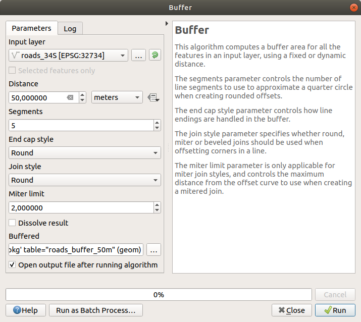
Кликните на Run, а затем закройте диалоговой окно Buffer.
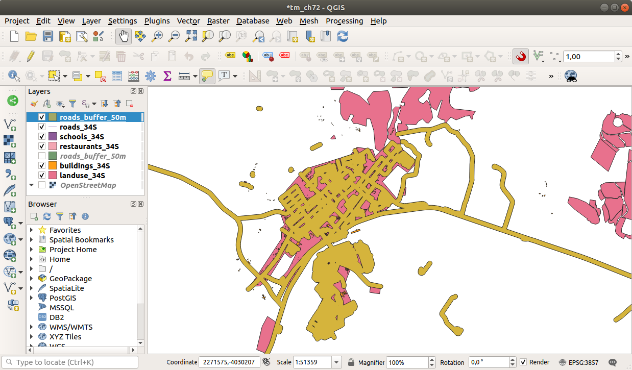
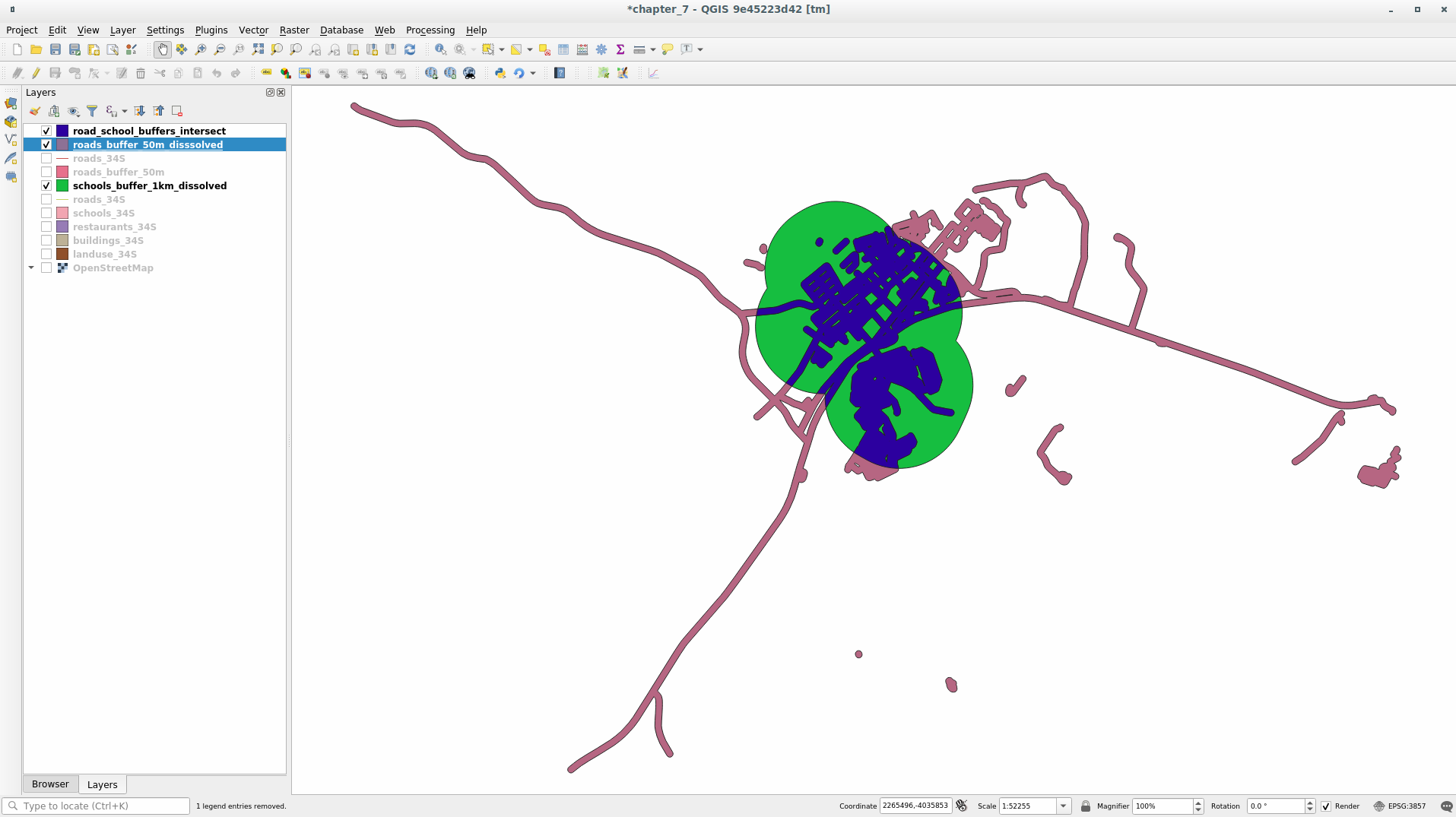
Ваша карта теперь будет выглядеть примерно так:
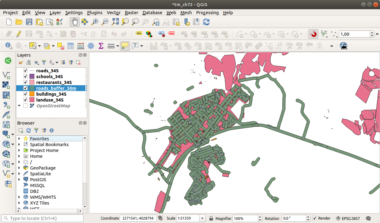
Если ваш новый слой находится в верхней части списка Layers, он, скорее всего, закроет большую часть вашей карты, но вы сможете увидеть все местности в вашем регионе, которые находятся на расстоянии в 50 м от дороги.
Обратите внимание, что в вашем буфере есть отдельные местности, соответствующие каждой отдельной дороге. Чтобы устранить эту проблему необходимо:
Uncheck the
roads_buffer_50mlayer and re-create the buffer with Dissolve results enabled.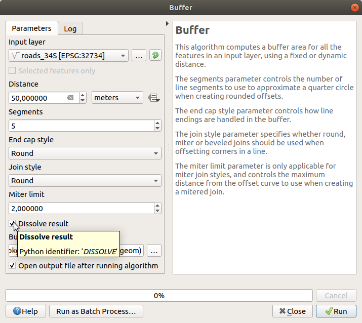
Save the output as
roads_buffer_50m_dissolvedКликните на Run и закройте диалоговой окно Buffer.
После того, как вы добавили слой в панель Layers, она будет выглядеть так:
Теперь лишних делений уже нет.
Примечание
Краткая справка (помощь) в правой части диалогового окна объясняет, как работает алгоритм. Если вам нужна дополнительная информация, просто кликните на кнопку Help в нижней части, чтобы открыть более подробное руководство по алгоритму.
6.2.7. ★☆☆ Try Yourself: Distance from schools
Следуйте тому же подходу, который описан выше, и создайте буфер для ваших школ.
It shall be 1 km in radius.
Save the new layer in the vector_analysis.gpkg file as schools_buffer_1km_dissolved.
Ответить
Your buffer dialog should look like this:
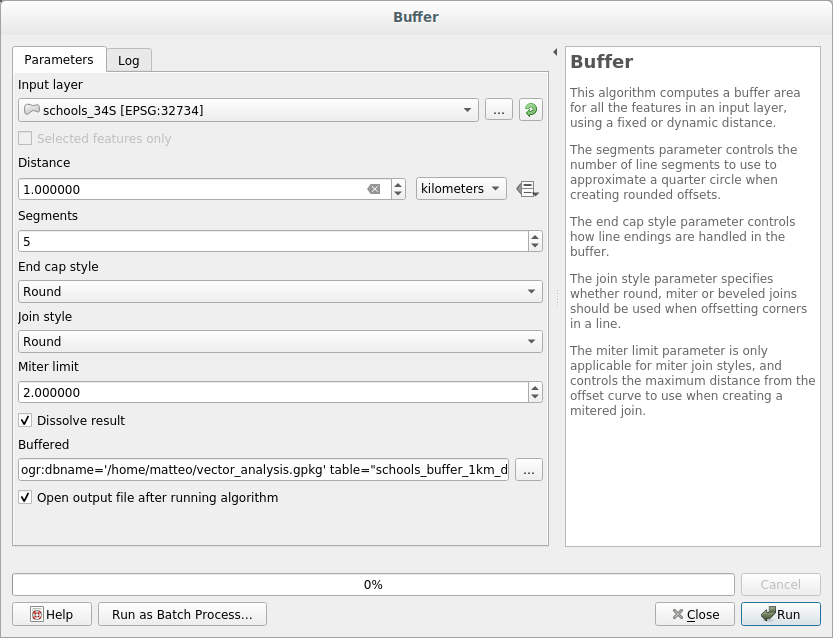
The Buffer distance is 1 kilometer.
The Segments to approximate value is set to
20. This is optional, but it’s recommended, because it makes the output buffers look smoother. Compare this: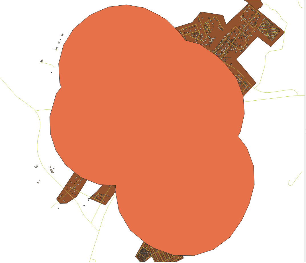
To this:
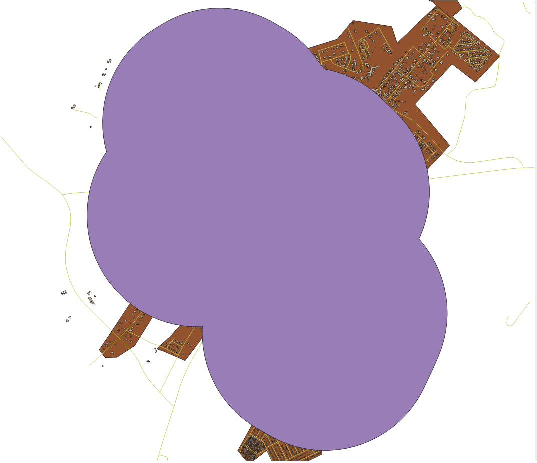
The first image shows the buffer with the Segments to approximate
value set to 5 and the second shows the value set to 20.
In our example, the difference is subtle, but you can see that the buffer’s edges
are smoother with the higher value.
6.2.8. ★☆☆ Follow Along: Overlapping Areas
Теперь мы определили местности, где дорога находится на расстоянии менее чем в 50 метрах, а также местности, расположенные от школы в пределах 1 км (по прямой линии, а не по дороге). Естественно нам нужны только те местности, которые отвечают обоим этим критериям. Для этого нам нужно будет использовать инструмент Intersect. Вы сможете найти его в группе в Processing Toolbox.
Используйте два буферных слоя как Input layer и Overlay layer выберите
vector_analysis.gpkgGeoPackage в Intersection с Layer nameroad_school_buffers_intersect. Остальное оставьте как предлагается (по умолчанию).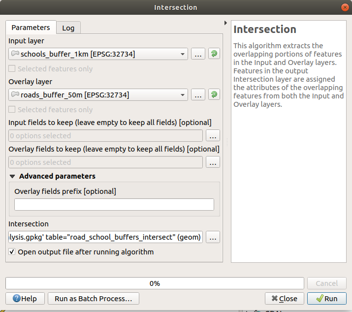
Кликните на кнопку Run.
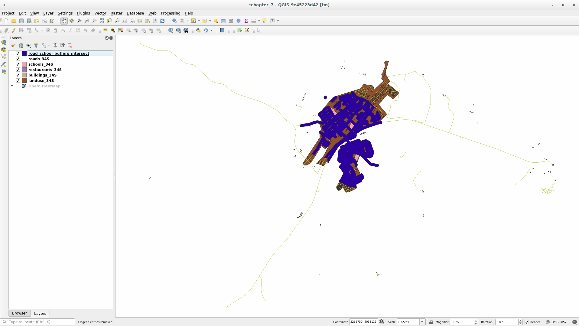
На изображении ниже местности, окрашенные синим цветом это те местности, где оба соответствия по критериям расстояния соблюдены.
Вы можете убрать два буферных слоя и оставить только тот, который показывает, где они перекрываются, так как мы действительно хотели это выяснить в первую очередь:
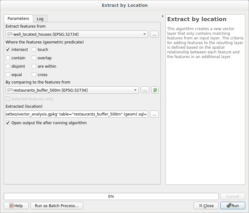
6.2.9. ★☆☆ Follow Along: Extract the Buildings
Теперь у вас есть местность, на которой здания должны перекрывать друг друга. Теперь вам надо извлечь здания в этой местности.
Ищите пункт в меню в Панели инструментов обработки.
Выберите
buildings_34Sв Extract features from. Проверьте intersect в Where the features (geometric predicate), выберите буферный слой пересечения в By comparing to the features from. Сохраните вvector_analysis.gpkgи назовите слойwell_located_houses.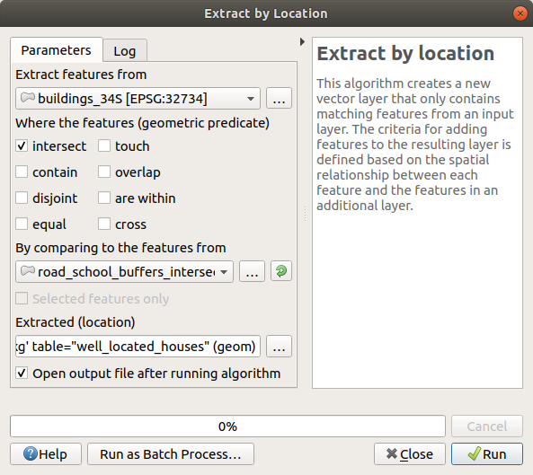
Кликните на кнопку Run и закройте диалоговое окно.
You will probably find that not much seems to have changed. If so, move the
well_located_houseslayer to the top of the layers list, then zoom in.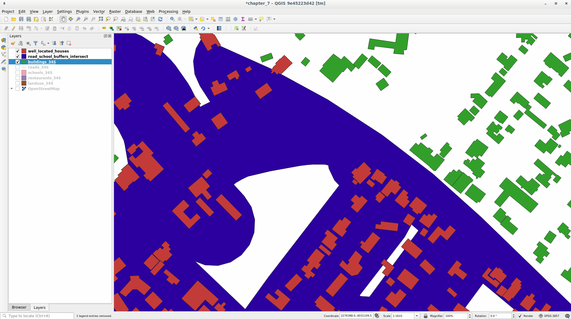
Здания красным цветом отвечают нашим критериям, а зеленым - нет.
Теперь у вас два отдельных слоя и вы сможете убрать
buildings_34Sиз списка слоев.
6.2.10. ★★☆ Try Yourself: Further Filter our Buildings
Теперь у нас есть слой, который показывает нам все здания в пределах 1 км от школы и в пределах 50 м от дороги. Нам теперь надо сократить этот отбор и показать только те здания, которые находятся в пределах 500 м от ресторана.
Using the processes described above, create a new layer called
houses_restaurants_500m which further filters your
well_located_houses layer to show only those which are
within 500m of a restaurant.
Ответить
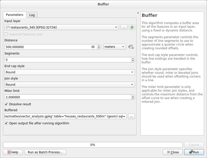
To create the new houses_restaurants_500m layer, we go through a two step
process:
First, create a buffer of 500m around the restaurants and add the layer to the map:
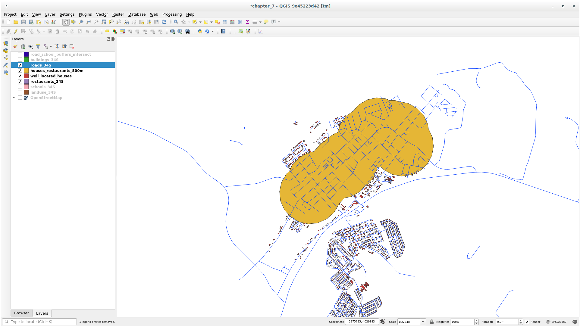
Next, extract buildings within that buffer area:
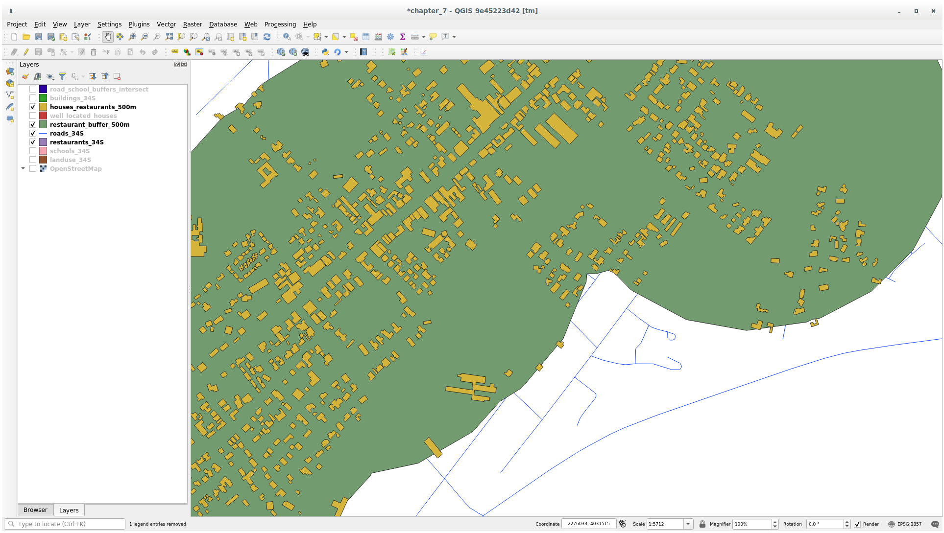
Your map should now show only those buildings which are within 50m of a road, 1km of a school and 500m of a restaurant:
6.2.11. ★☆☆ Follow Along: Select Buildings of the Right Size
Чтобы увидеть, какие здания имеют правильный размер (более 100 квадратных метров), нам надо рассчитать их размер.
Select the
houses_restaurants_500mlayer and open the Field Calculator by clicking on the Open Field Calculator button in the main toolbar or in
the attribute table window
Open Field Calculator button in the main toolbar or in
the attribute table windowВыберите Create a new field, установите Output field name на
AREA, выберите Decimal number (real) как Output field type, и выберите$areaиз группы .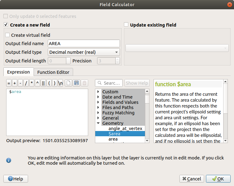
В новом поле
AREAбудет площадь каждого здания в квадратных метрах.Кликните на OK. Поле
AREAдобавлено в конце таблицы атрибутов.Кликните мышкой на кнопку
 Toggle Editing для того, чтобы завершить редактирование и сохраните ваши изменения при появлении запроса.
Во вкладке в свойствах слоя установите Provider Feature Filter на
"AREA >= 100.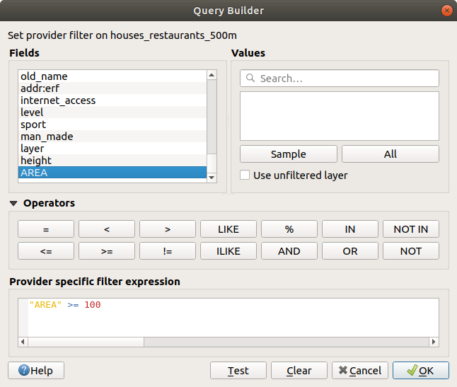
Кликните на кнопку OK.
Ваша карта теперь должна показывать только те здания, которые соответствуют нашим первоначальным критериям и имеют размер более 100 квадратных метров.
6.2.12. ★☆☆ Попробуй себя:
Сохраните ваш вариант как новый слой, следуя подходу, которому вы научились выше. Файл должен быть сохранен внутри той же базы данных GeoPackage с названием solution.
6.2.13. В заключение
Следуя подходу решения проблем GIS вместе с инструментами векторного анализа QGIS, вы смогли быстро и легко решить проблему с несколькими критериями.
6.2.14. Что дальше?
На следующем уроке мы изучим, как рассчитать наикратчайшее расстояние по дорогам от одной точки до другой.