17.25. More iterative execution of algorithms
Note
This lesson shows how to combine the iterative execution of algorithms with the modeler to get more automation.
The iterative execution of algorithms is available not just for built-in algorithms, but also for the algorithms that you can create yourself, such as models. We are going to see how to combine a model and the iterative execution of algorithms, so we can obtain more complex results with ease.
The data the we are going to use for this lesson is the same one that we already used for the last one. In this case, instead of just clipping the DEM with each watershed polygon, we will add some extra steps and calculate a hypsometric curve for each of them, to study how elevation is distributed within the watershed.
Since we have a workflow that involves several steps (clipping + computing the hypsometric curve), we should go to the modeler and create the corresponding model for that workflow.
You can find the model already created in the data folder for this lesson, but it would be good if you first try to create it yourself. The clipped layer is not a final result in this case, since we are just interested in the curves, so this model will not generated any layers, but just a table with the curve data.
The model should look like this:
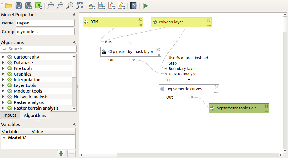
Add the model to you models folder, so it is available in the toolbox, and execute it.
Select the DEM and watersheds basins.
The algorithm will generate tables for all the basins and place them in the output directory.
We can make this example more complex by extending the model and computing some slope statistics. Add the Slope algorithm to the model, and then the Raster statistics algorithm, which should use the slope output as its only input.
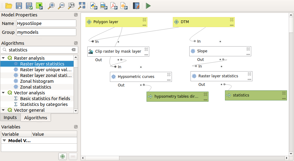
If you now run the model, apart from the tables you will get a set of pages with statistics. These pages will be available in the results dialog.