18.4. Rodando o nosso primeiro algoritmo. A caixa de ferramentas
Nota
Nesta lição, vamos executar o nosso primeiro algoritmo e conseguir o nosso primeiro resultado a partir disso.
Como já mencionado, a estrutura de processamento pode executar algoritmos de outras aplicações, mas também contém algoritmos nativos que não precisam de software externo para serem executados. Para começar a explorar a estrutura de processamento, nós iremos executar um desses algoritmos nativos. Em particular, vamos calcular os centróides de um conjunto de polígonos.
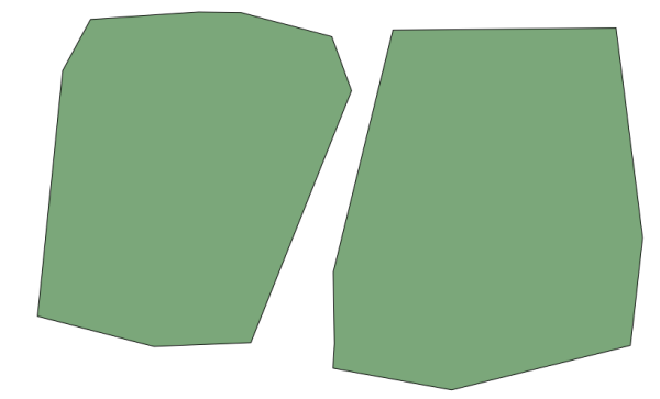
Primeiro, abra o projeto QGIS correspondente a esta lição. Ele contém apenas uma única camada com dois polígonos
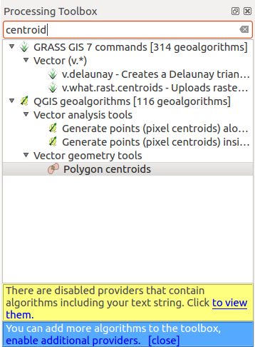
Now go to the text box at the top of the toolbox. That is the search box, and if you type text in it, it will filter the list of algorithms so just those ones containing the entered text are shown. If there are algorithms that match your search but belong to a provider that is not active, an additional label will be shown in the lower part of the toolbox.
Type centroids and you should see something like this.
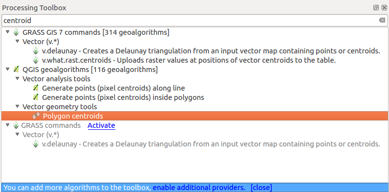
The search box is a very practical way of finding the algorithm you are looking for. At the bottom of the dialog, an additional label shows that there are algorithms that match your search but belong to a provider that is not active. If you click on the link in that label, the list of algorithms will also include results from those inactive providers, which will be shown in light gray. A link to activate each inactive provider is also shown. We’ll see later how to activate other providers.
To execute an algorithm, you just have to double-click on its name in the toolbox. When you double-click on the Polygon centroids algorithm, you will see the following dialog.
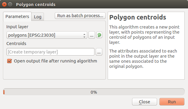
All algorithms have a similar interface, which basically contains input parameters that you have to fill, and outputs that you have to select where to store. In this case, the only input we have is a vector layer with polygons.
Select the Polygons layer as input. The algorithm has a single output, which is the centroids layer. There are two options to define where a data output is saved: enter a filepath or save it to a temporary filename
In case you want to set a destination and not save the result in a temporary file, the format of the output is defined by the filename extension. To select a format, just select the corresponding file extension (or add it if you are directly typing the filepath instead). If the extension of the filepath you entered does not match any of the supported ones, a default extension (usually .dbf for tables, .tif for raster layers and .shp for vector ones) will be appended to the filepath and the file format corresponding to that extension will be used to save the layer or table.
Em todos os exercícios deste guia salvaremos os resultados em um arquivo temporário, já que não há necessidade de guardá-los para uso posterior. Sinta-se livre para salvá-los para um local permanente se você quiser.
Aviso
Temporary files are deleted once you close QGIS. If you create a project with an output that was saved as a temporary output, QGIS will complain when you try to open back the project later, since that output file will not exist.
Once you have configured the algorithm dialog, press [Run] to run the algorithm.
Você terá o seguinte resultado:
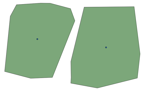
A saída tem o mesmo SRC que a entrada. Os Geoalgoritimos assumem que todas as camadas de entrada compartilham o mesmo SRC e não realiza nenhuma reprojeção. Exceto no caso de alguns algoritmos especiais (por exemplo, os de reprojeção), as saídas também terão o mesmo SRC. Veremos mais sobre isso em breve.
Try yourself saving it using different file formats (use, for instance, shp and geojson as extensions). Also, if you do not want the layer to be loaded in QGIS after it is generated, you can check off the checkbox that is found below the output path box.