7.2. Lesson: Vectoranalyse
Vectorgegevens kunnen ook worden geanalyseerd om te onthullen hoe verschillende objecten met elkaar omgaan in de ruimte. Er zijn vele aan analyse gerelateerde functies in GIS, dus zullen we ze niet allemaal behandelen. In plaats daarvan zullen we een vraag stellen en die proberen op te lossen met behulp van de gereedschappen die QGIS verschaft.
Het doel voor deze les. Een vraag stellen en die beantwoorden met behulp van gereedschappen voor analyse.
7.2.1.  Het proces GIS
Vóór we beginnen zou het handig zijn om een kort overzicht te geven van een proces dat gebruikt kan worden om elk probleem in GIS op te lossen. De manier om dat te doen is:
Benoem het probleem
Haal de gegevens op
Analyseer het probleem
Geef de resultaten weer
7.2.2. The problem
Laten we het proces beginnen door een probleem te benoemen om op te lossen. U bent bijvoorbeeld een makelaar en u zoekt naar een woning in Swellendam voor cliënten die de volgende criteria hebben:
- It needs to be in Swellendam.
- It must be within reasonable driving distance of a school (say 1km).
- It must be more than 100m squared in size.
- Closer than 50m to a main road.
- Closer than 500m to a restaurant.
7.2.3. The data
We hebben de volgende gegevens nodig om deze vragen te kunnen beantwoorden:
- The residential properties (buildings) in the area.
- The roads in and around the town.
- The location of schools and restaurants.
- The size of buildings.
All of this data is available through OSM and you should find that the dataset you have been using throughout this manual can also be used for this lesson. However, in order to ensure we have the complete data, we will re-download the data from OSM using QGIS’ built-in OSM download tool.
Notitie
Hoewel downloads van OSM consistente velden voor de gegevens hebben, kunnen de bedekking en de details variëren. Als u ziet dat de door u gekozen regio, bijvoorbeeld, geen informatie bevat over restaurants, zou u misschien een andere regio moeten kiezen.
7.2.4. Follow Along: Start a Project
- Start a new QGIS project.
- Use the OpenStreetMap data download tool found in the Vector ‣ OpenStreetMap menu to download the data for your chosen region.
- Save the data as osm_data.osm in your exercise_data folder.
- Note that the osm format is a type of vector data. Add this data as a vector layer as usually Layer ‣ Add vector layer..., browse to the new osm_data.osm file you just downloaded. You may need to select Show All Files as the file format.
- Select osm_data.osm and click Open
- In the dialog which opens, select all the layers, except the other_relations and multilinestrings layer:
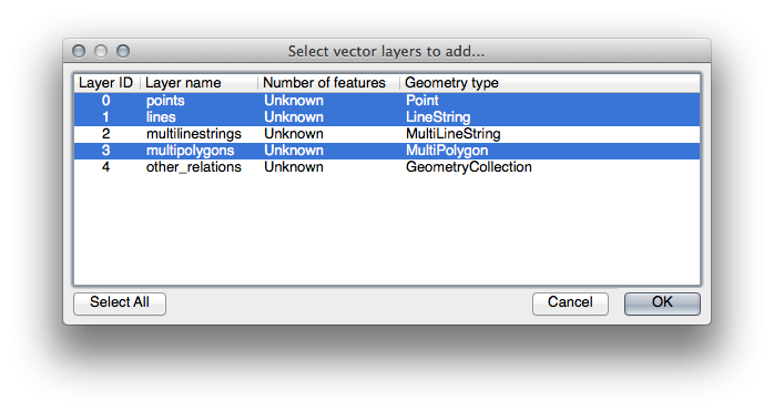
This will import the OSM data as separate layers into your map.
The data you just downloaded from OSM is in a geographic coordinate system, WGS84, which uses latitude and longitude coordinates, as you know from the previous lesson. You also learnt that to calculate distances in meters, we need to work with a projected coordinate system. Start by setting your project’s coordinate system to a suitable CRS for your data, in the case of Swellendam, WGS 84 / UTM zone 34S:
- Open the Project Properties dialog, select CRS and filter the list to find WGS 84 / UTM zone 34S.
Klik op OK.
We now need to extract the information we need from the OSM dataset. We need to end up with layers representing all the houses, schools, restaurants and roads in the region. That information is inside the multipolygons layer and can be extracted using the information in its Attribute Table. We’ll start with the schools layer:
- Right-click on the multipolygons layer in the Layers list and open the Layer Properties.
- Go to the General menu.
- Under Feature subset click on the [Query Builder] button to open the Query builder dialog.
- In the Fields list on the left of this dialog until you see the field amenity.
- Click on it once.
- Click the All button underneath the Values list:
Now we need to tell QGIS to only show us the polygons where the value of amenity is equal to school.
- Double-click the word amenity in the Fields list.
- Watch what happens in the Provider specific filter expression field below:
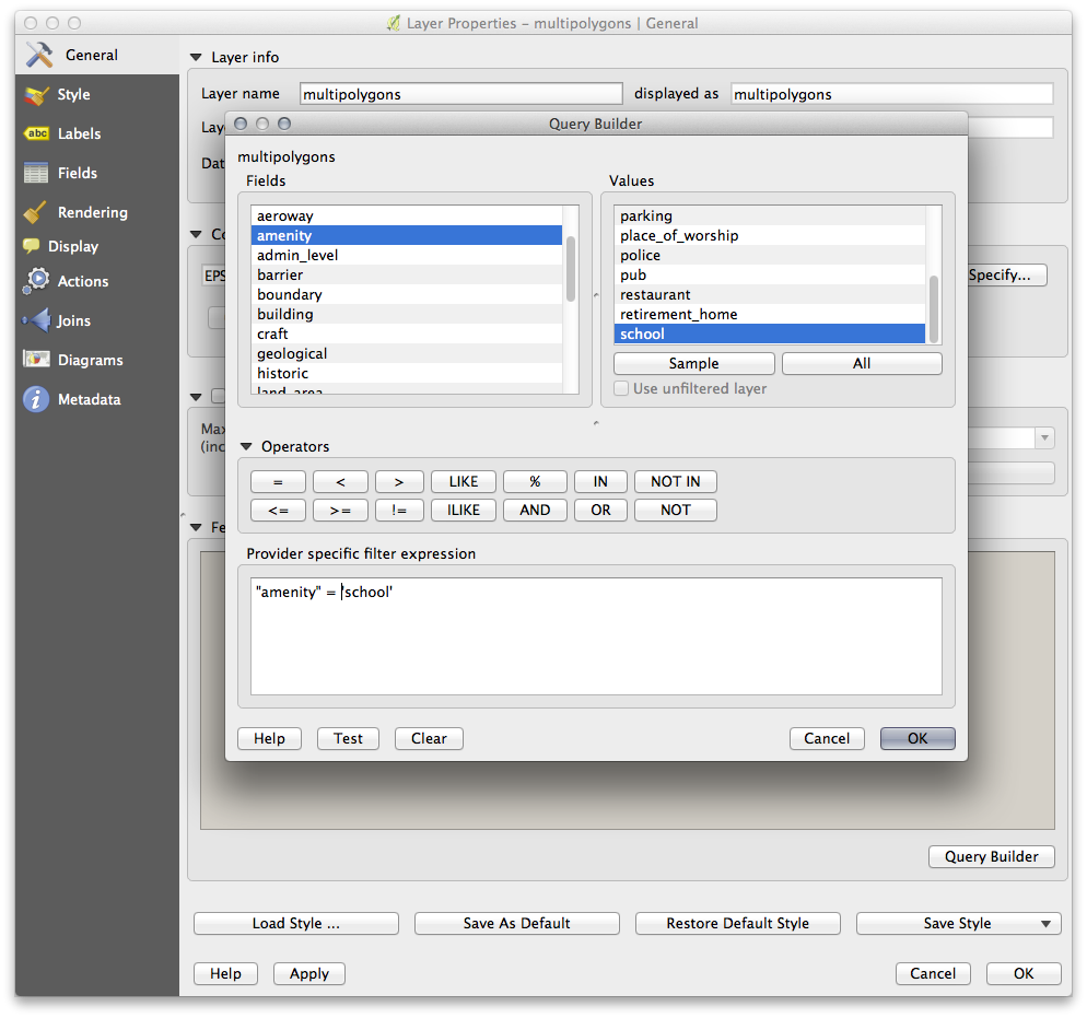
The word "amenity" has appeared. To build the rest of the query:
- Click the = button (under Operators).
- Double-click the value school in the Values list.
- Click OK twice.
This will filter OSM’s multipolygons layer to only show the schools in your region. You can now either:
- Rename the filtered OSM layer to schools and re-import the multipolygons layer from osm_data.osm, OR
- Duplicate the filtered layer, rename the copy, clear the Query Builder and create your new query in the Query Builder.
7.2.5.  Try Yourself Extract Required Layers from OSM
Using the above technique, use the Query Builder tool to extract the remaining data from OSM to create the following layers:
- roads (from OSM’s lines layer)
- restaurants (from OSM’s multipolygons layer)
- houses (from OSM’s multipolygons layer)
You may wish to re-use the roads.shp layer you created in earlier lessons.
- Save your map under exercise_data, as analysis.qgs (this map will be used in future modules).
- In your operating system’s file manager, create a new folder under exercise_data and call it residential_development. This is where you’ll save the datasets that will be the results of the analysis functions.
7.2.6. Try Yourself Find important roads
Some of the roads in OSM’s dataset are listed as unclassified, tracks, path and footway. We want to exclude these from our roads dataset.
Open the Query Builder for the roads layer, click Clear and build the following query:
"highway" != 'NULL' AND "highway" != 'unclassified' AND "highway" != 'track' AND "highway" != 'path' AND "highway" != 'footway'
You can either use the approach above, where you double-clicked values and clicked buttons, or you can copy and paste the command above.
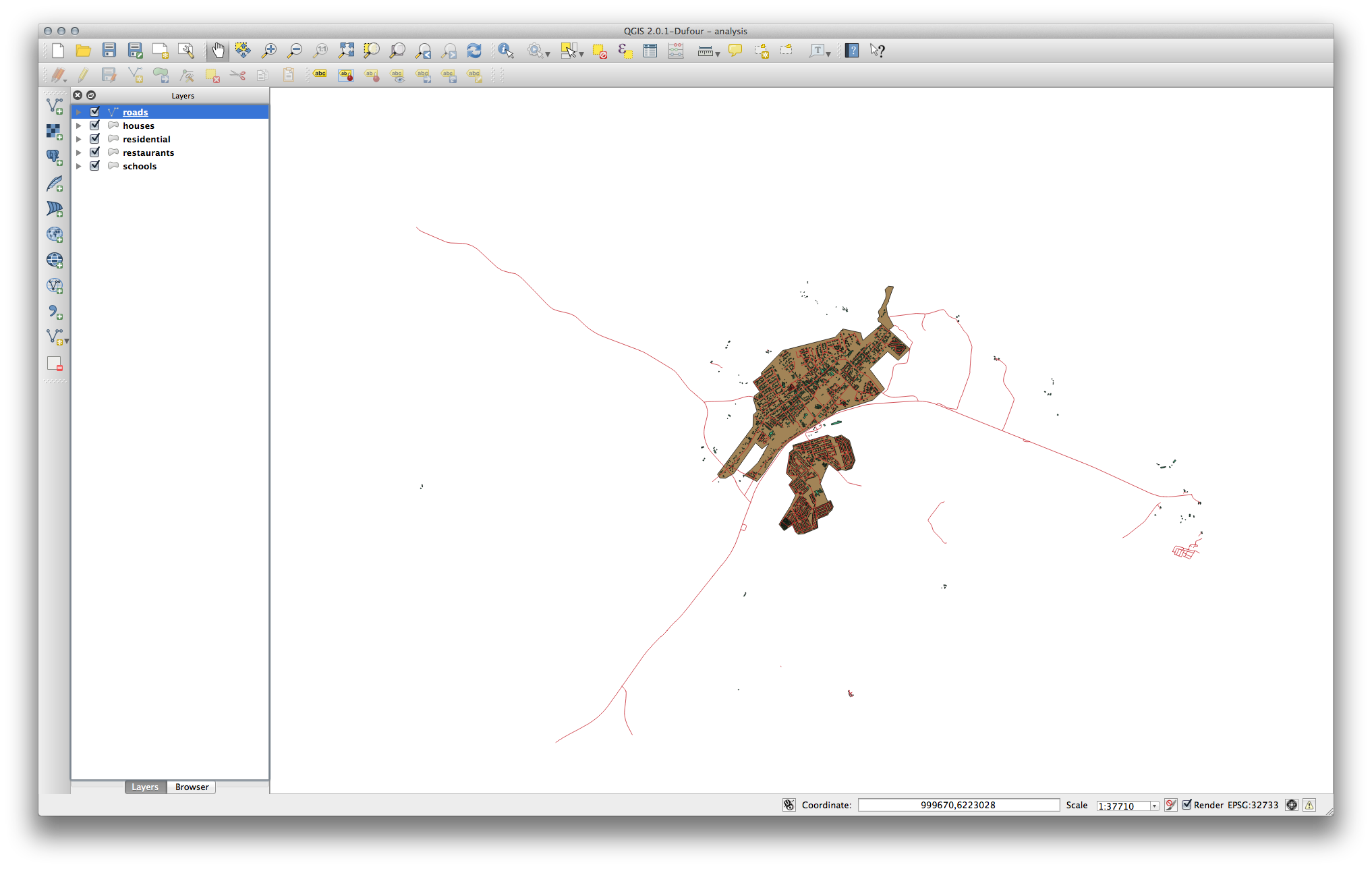
This should immediately reduce the number of roads on your map:
7.2.7. Try Yourself CRS van een laag converteren
Because we are going to be measuring distances within our layers, we need to change the layers’ CRS. To do this, we need to select each layer in turn, save the layer to a new shapefile with our new projection, then import that new layer into our map.
Notitie
In dit voorbeeld gebruiken we het CRS WGS 84 / UTM zone 34S, maar u kunt een UTM CRS gebruiken dat meer toepasselijk is voor uw regio.
- Right click the roads layer in the Layers panel.
- Click Save as...
- In the Save Vector As dialog, choose the following settings and click Ok (making sure you select Add saved file to map):
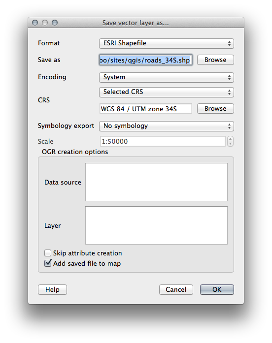
The new shapefile will be created and the resulting layer added to your map.
Notitie
If you don’t have activated Enable ‘on the fly’ CRS transformation or the Automatically enable ‘on the fly’ reprojection if layers have different CRS settings (see previous lesson), you might not be able to see the new layers you just added to the map. In this case, you can focus the map on any of the layers by right click on any layer and click Zoom to layer extent, or just enable any of the mentioned ‘on the fly’ options.
- Remove the old roads layer.
Repeat this process for each layer, creating a new shapefile and layer with “_34S” appended to the original name and removing each of the old layers.
Als u eenmaal het proces voor elke laag heeft voltooid, klik dan met rechts op een laag en klik op Zoom naar laag om de kaart te focussen op het gebied waarin we geïnteresseerd zijn.
Nu we de gegevens van OSM hebben geconverteerd naar een UTM-projectie, kunnen we onze berekeningen beginnen.
7.2.8. Follow Along: Analyseren van het probleem: Afstanden van scholen en wegen
QGIS stelt u in staat afstanden te berekenen vanaf elk vectorobject.
- Make sure that only the roads_34S and houses_34S layers are visible, to simplify the map while you’re working.
- Click on the Vector ‣ Geoprocessing Tools ‣ Fixed distance buffer tool:
This gives you a new dialog.
Stel dat als volgt in:
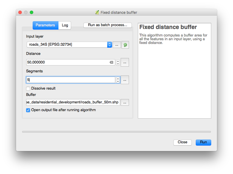
The Distance is in meters because our input dataset is in a Projected Coordinate System that uses meter as its basic measurement unit. This is why we needed to use projected data.
- Save the resulting layer under exercise_data/residential_development/ as roads_buffer_50m.shp.
- Click OK and it will create the buffer.
- When it asks you if it should “add the new layer to the TOC”, click Yes. (“TOC” stands for “Table of Contents”, by which it means the Layers list).
- Close the Fixed distance buffer dialog.
Nu zal uw kaart er ongeveer zo uitzien:
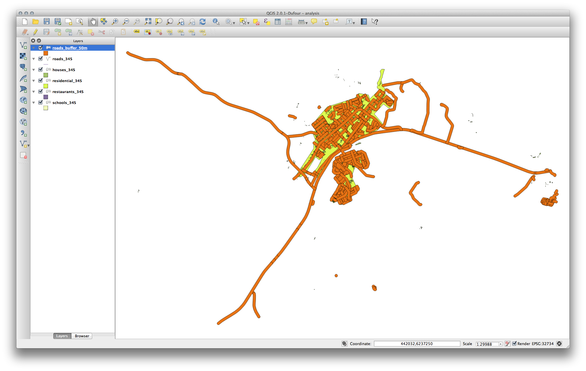
If your new layer is at the top of the Layers list, it will probably obscure much of your map, but this gives us all the areas in your region which are within 50m of a road.
However, you’ll notice that there are distinct areas within our buffer, which correspond to all the individual roads. To get rid of this problem, remove the layer and re-create the buffer using the settings shown here:
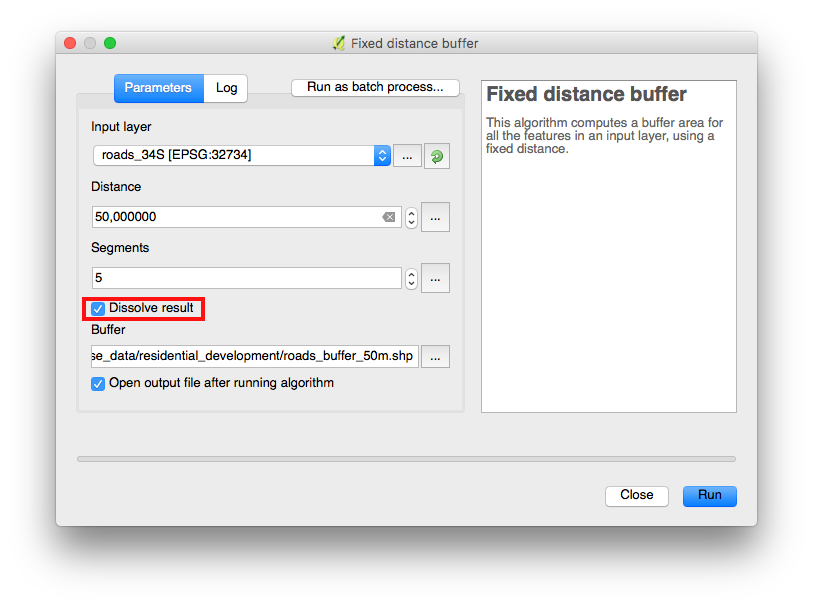
- Note that we’re now checking the Dissolve result box.
- Save the output under the same name as before (click Yes when it asks your permission to overwrite the old one).
- Click OK and close the Fixed distance buffer dialog again.
Once you’ve added the layer to the Layers list, it will look like this:
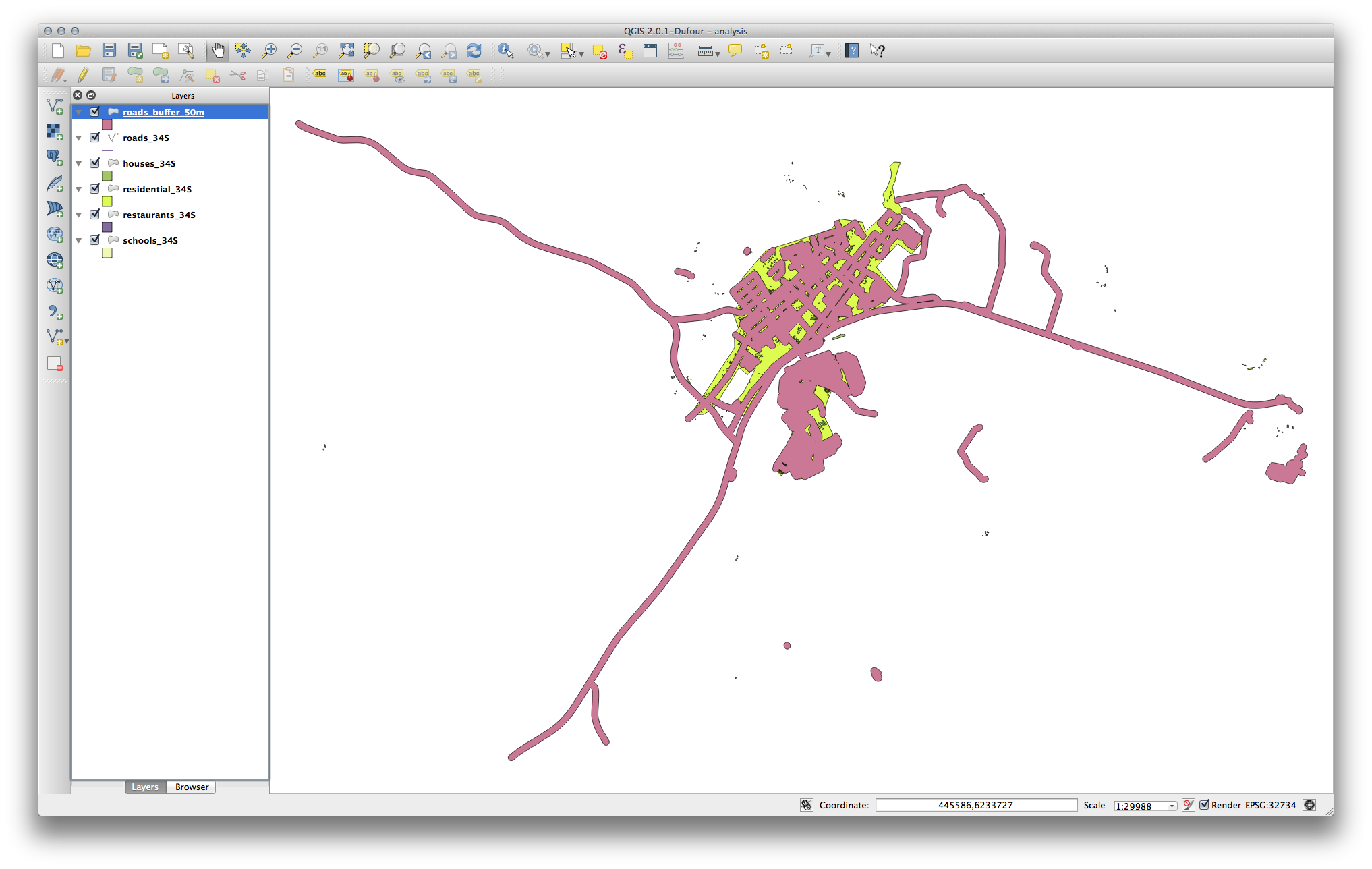
Nu zijn er geen onnodige onderverdelingen meer.
7.2.9. Try Yourself Afstand van scholen
Gebruik dezelfde benadering als hierboven en maak een buffer voor uw scholen.
It needs to be 1 km in radius, and saved under the usual directory as schools_buffer_1km.shp.
7.2.10. Follow Along: Overlappende gebieden
Now we have areas where the road is 50 meters away and there’s a school within 1 km (direct line, not by road). But obviously, we only want the areas where both of these criteria are satisfied. To do that, we’ll need to use the Intersect tool. Find it under Vector ‣ Geoprocessing Tools ‣ Intersect. Set it up like this:
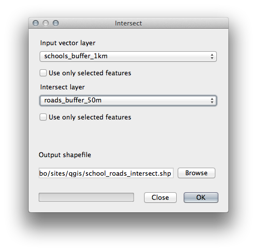
The two input layers are the two buffers; the save location is as usual; and the file name is road_school_buffers_intersect.shp. Once it’s set up like this, click OK and add the layer to the Layers list when prompted.
In de afbeelding hieronder geven de blauwe gebieden aan waar in één keer aan beide criteria voor de afstand wordt voldaan!
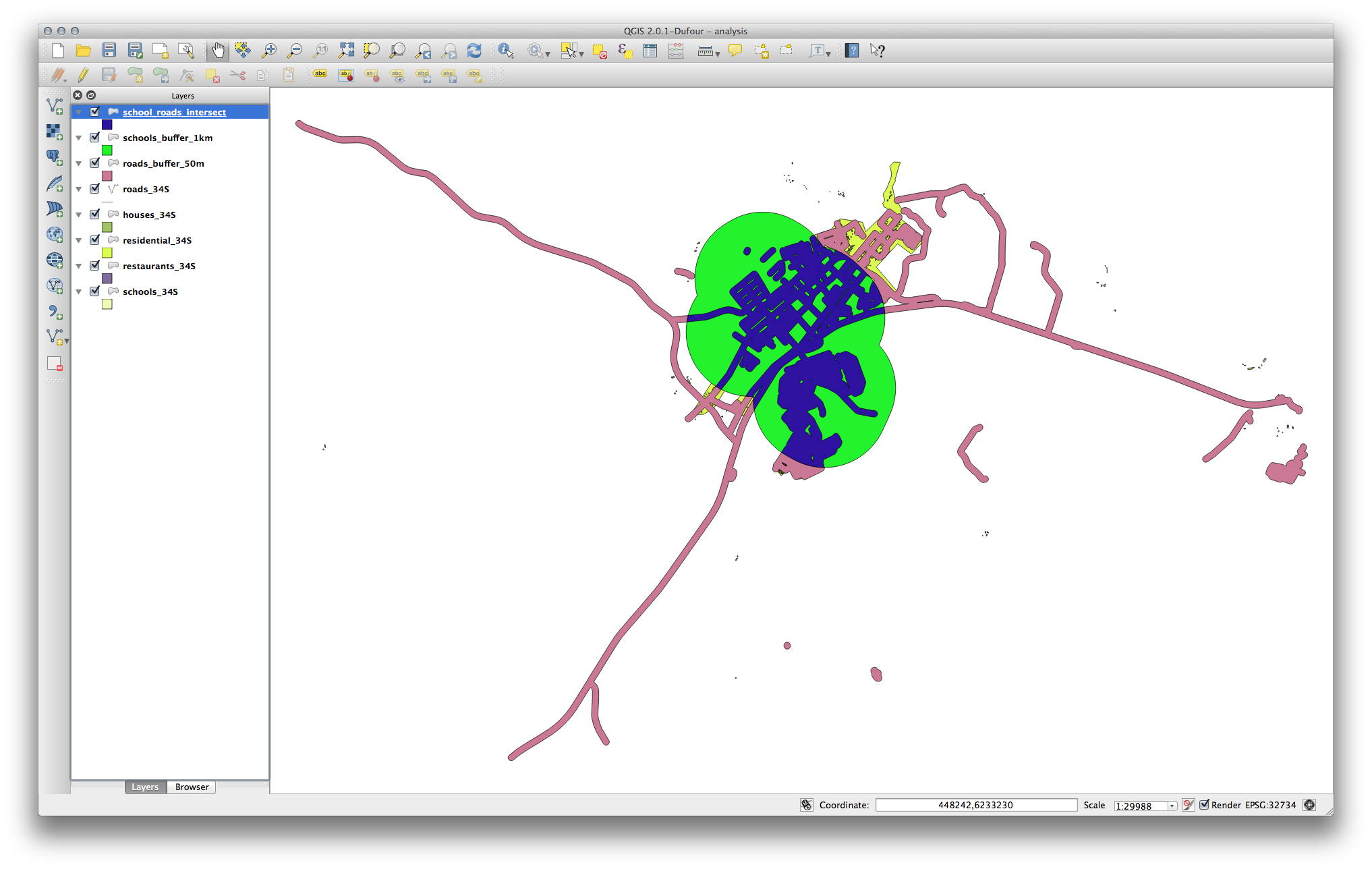
U kunt de twee bufferlagen verwijderen en alleen die ene behouden waar zij overlappen, omdat dat is wat we in eerste instantie echt wilden weten:
7.2.11. Follow Along: Select the Buildings
Now you’ve got the area that the buildings must overlap. Next, you want to select the buildings in that area.
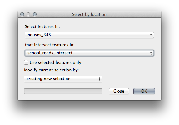
- Click on the menu entry Vector ‣ Research Tools ‣ Select by location. A dialog will appear.
Stel dat als volgt in:
- Click OK, then Close.
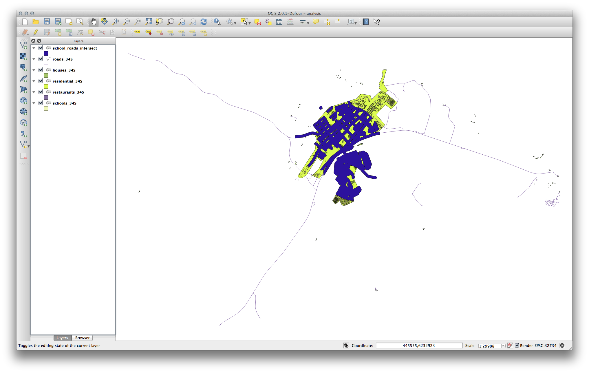
- You’ll probably find that not much seems to have changed. If so, move the school_roads_intersect layer to the bottom of the layers list, then zoom in:
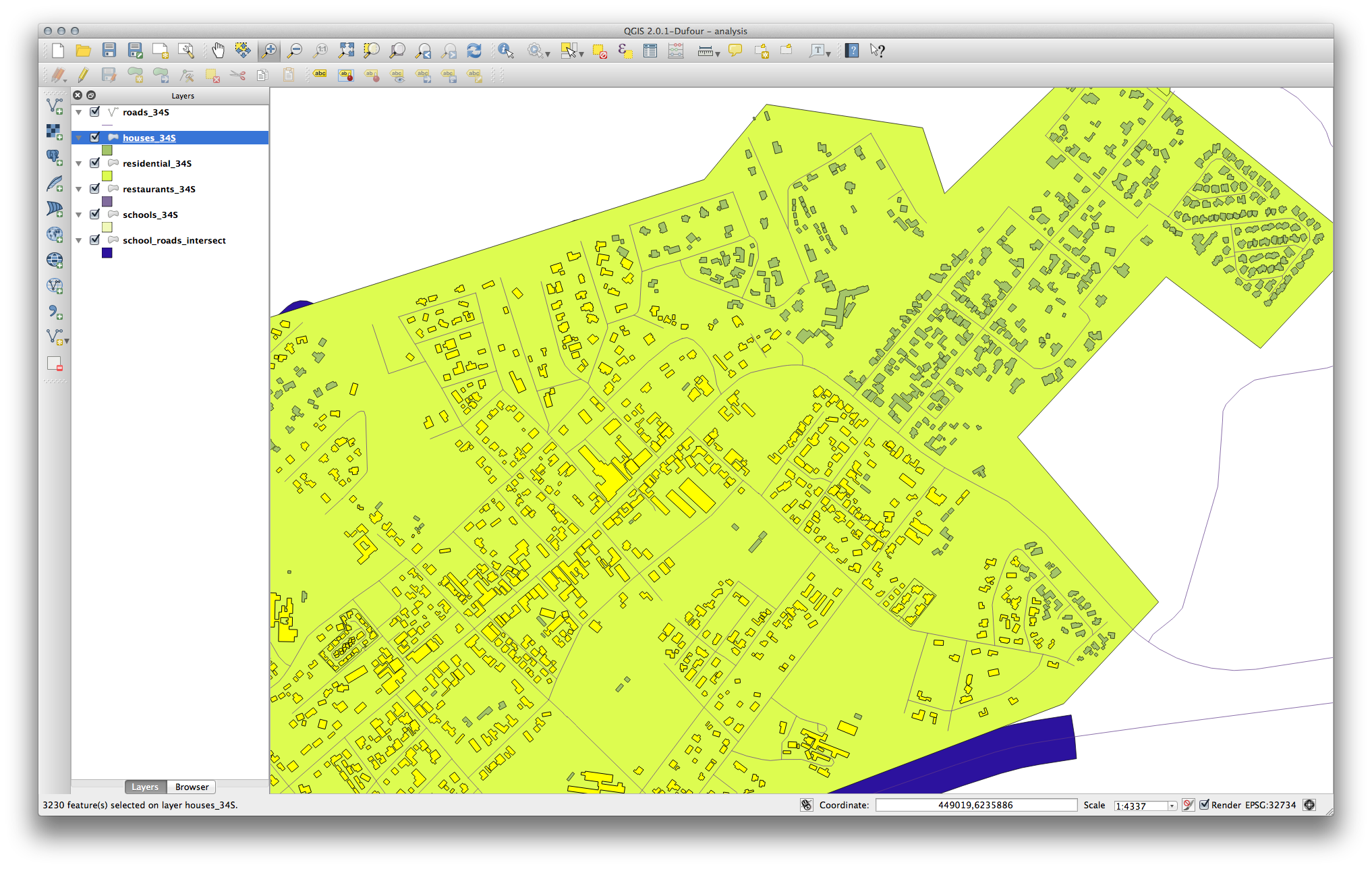
The buildings highlighted in yellow are those which match our criteria and are selected, while the buildings in green are those which do not. We can now save the selected buildings as a new layer.
- Right-click on the houses_34S layer in the Layers list.
- Select Save Selection As....
- Set the dialog up like this:
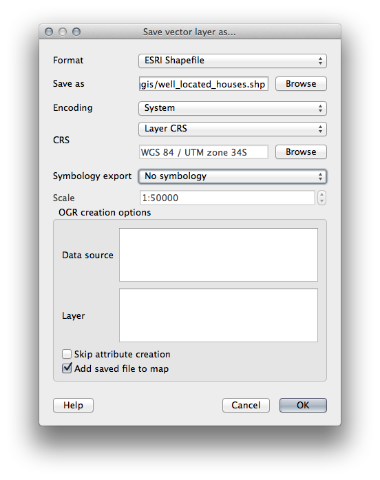
- The file name is well_located_houses.shp.
Klik op OK.
Now you have the selection as a separate layer and can remove the houses_34S layer.
7.2.12. Try Yourself Onze gebouwen verder filteren
We hebben nu een laag die ons alle gebouwen binnen 1 km van een school en binnen 50 m vanaf een weg toont. We moeten nu die selectie verkleinen om ons alleen gebouwen te tonen die binnen 500 m vanaf een restaurant liggen.
Using the processes described above, create a new layer called houses_restaurants_500m which further filters your well_located_houses layer to show only those which are within 500m of a restaurant.
7.2.13. Follow Along: Selecteren van gebouwen met de juiste grootte
To see which buildings are the correct size (more than 100 square meters), we first need to calculate their size.
- Open the attribute table for the houses_restaurants_500m layer.
- Enter edit mode and open the field calculator.
Stel dat als volgt in:
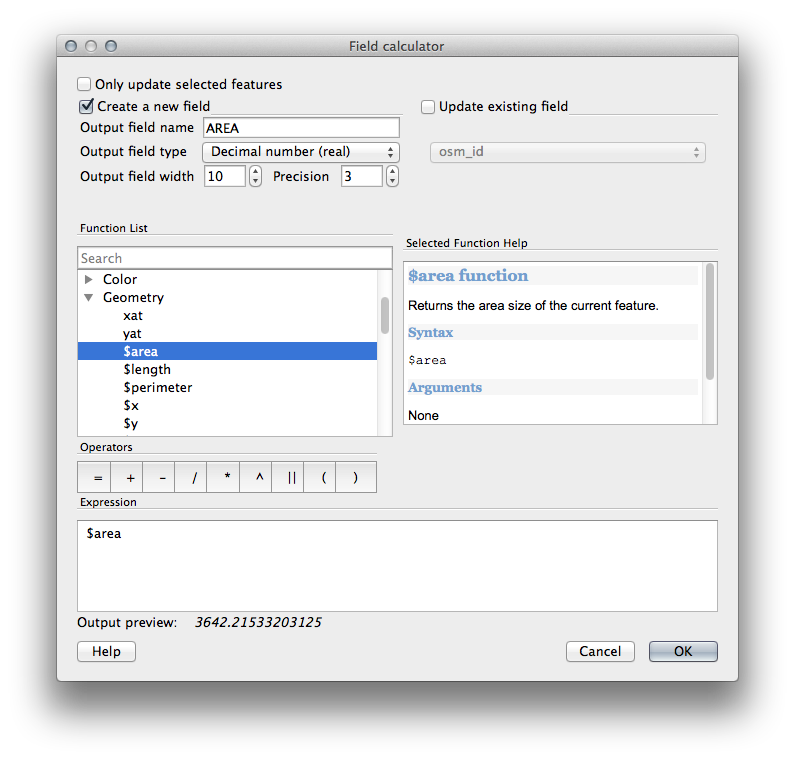
- If you can’t find AREA in the list, try creating a new field as you did in the previous lesson of this module.
Klik op OK.
- Scroll to the right of the attribute table; your AREA field now has areas in metres for all the buildings in your houses_restaurants_500m layer.
Klik opnieuw op de knop voor de modus Bewerken om het bewerken te voltooien en sla uw gegevens op als daarnaar gevraagd wordt.
- Build a query as earlier in this lesson:
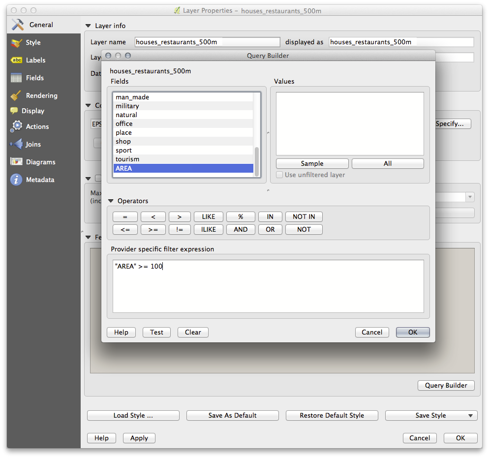
- Click OK. Your map should now only show you those buildings which match our starting criteria and which are more than 100m squared in size.
7.2.14. Try Yourself
- Save your solution as a new layer, using the approach you learned above for doing so. The file should be saved under the usual directory, with the name solution.shp.
7.2.15. In Conclusion
Met behulp van de benadering van probleemoplossing voor GIS, tezamen met de gereedschappen voor vectoranalyse van QGIS, was u in staat een probleem met meerdere criteria snel een gemakkelijk op te lossen.
7.2.16. What’s Next?
In de volgende les, zullen we kijken naar de berekening van de kortste afstand over de weg van het ene punt naar een ander.