Importante
A tradução é um esforço comunitário você pode contribuir. Esta página está atualmente traduzida em 67.85%.
12.2. Trabalhando com a tabela de atributos
A tabela de atributos exibe informações sobre as feições de uma camada selecionada. Cada linha da tabela representa uma feição (com ou sem geometria) e cada coluna contém uma informação específica sobre a feição. As feições da tabela podem ser pesquisadas, selecionadas, movidas ou mesmo editadas.
12.2.1. Prefácio: Tabelas espaciais e não espaciais
QGIS allows you to load spatial and non-spatial layers. This currently includes tables supported by GDAL and delimited text, as well as the PostgreSQL, MS SQL Server, SpatiaLite and Oracle providers. All loaded layers are listed in the Layers panel. Whether a layer is spatially enabled or not determines whether you can interact with it on the map.
As tabelas não espaciais podem ser navegadas e editadas usando a visualização da tabela de atributos. Além disso, eles podem ser usados para pesquisas de campo. Por exemplo, você pode usar colunas de uma tabela não espacial para definir valores de atributos ou um intervalo de valores permitidos para serem adicionados a uma camada vetorial específica durante a digitalização. Dê uma olhada no widget de edição na seção Propriedades do formulário de atributos para descobrir mais.
12.2.2. Apresentando a Interface da Tabela de Atributos
Para abrir a tabela de atributos para uma camada vetorial, ative a camada clicando nela Painel Camadas. Em seguida, no menu principal: seleção de menus: menu Camada, escolha  :menuselection: Abrir tabela de atributos. Também é possível clicar com o botão direito do mouse na camada e escolher no menu suspenso ou clique em :guilabel: botão Abrir tabela de atributos na barra de ferramentas Atributos. Se você preferir atalhos, F6 abrirá a tabela de atributos. Shift+F6 abrirá a tabela de atributos filtrada para os recursos selecionados e: kbd:Ctrl+F6 abrirá a tabela de atributos filtrados para os recursos visíveis.
Isso abrirá uma nova janela que exibe os atributos da feição para a camada (figure_attributes_table). De acordo com a configuração em :menuselection: menu Configurações –> Opções –> Fonte de dados, a tabela de atributos será aberta em uma janela encaixada ou em uma janela regular. O número total de feições na camada e o número de feições atualmente selecionados/filtrados são mostrados no título da tabela de atributos, bem como se a camada é espacialmente limitada.
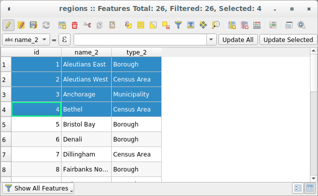
Fig. 12.73 Tabela de atributos para a camada de regiões
Os botões na parte superior da janela da tabela de atributos fornecem a seguinte funcionalidade:
Ícone |
Etiqueta |
Finalidade |
Atalho Padrão |
|---|---|---|---|
|
Alternar modo de edição |
Habilitar funcionalidades de edição |
Ctrl+E |
|
Alternar modo multi edição |
Atualize vários campos de várias feições |
|
|
Salvar Edições |
Salvar modificações atuais |
|
|
Recarregar a tabela |
||
|
Adicionar feição |
Adicionar nova feição sem geometria |
|
|
Add feature via attribute table |
Inserts a new empty row in the attribute table to be filled in |
|
|
Add feature via attribute form |
Opens the feature attributes form for data entry |
|
|
Excluir feições selecionadas |
Remover feições selecionadas para a camada |
|
|
Cortar feições selecionadas para área de transferência |
Ctrl+X |
|
|
Copiar feições selecionadas para a área de transferência |
Ctrl+C |
|
|
Colar feições da área de transferência |
Inserir novas feições das copiadas |
Ctrl+V |
|
Selecionar feições usando uma expressão |
||
|
Selecionar Todas |
Selecionar todas feições em uma camada |
Ctrl+A |
|
Seleção invertida |
Inverter a seleção atual na camada |
Ctrl+R |
|
Desselecionar todas |
Desselecionar todas as feições na camada atual |
Ctrl+Shift+A |
|
Filtrar/Selecionar feições usando formulário |
Ctrl+F |
|
|
Mover selecionadas para o topo |
Mover linhas selecionadas para o todo da tabela |
|
|
Mapa panorâmico para selecionar linhas |
Ctrl+P |
|
|
Aproximar mapa para selecionar linhas |
Ctrl+J |
|
|
Novo campo |
Adicionar um novo campo para uma fonte de dados |
Ctrl+W |
|
Excluir campo |
Remover um campo a partir da fonte de dados |
|
|
Organizar colunas |
Mostrar/ocultar campos da tabela de atributos |
|
|
Abrir calculadora de campo |
Atualização de campo para muitas feições em uma linha |
Ctrl+I |
|
Formatação condicional |
Ativar formatação de tabela |
|
|
Tabela de Atributos do Dock |
Permite encaixar/desencaixar a tabela de atributos |
|
|
Actions |
Listas de ações relatadas para uma camada |


Atenção
Depending on the format of the data and the GDAL library built with your QGIS version, some tools may not be available.
Abaixo desses botões está a barra Cálculo de campo rápido (ativada apenas em modo de edição), que permite aplicar rapidamente cálculos a todos ou parte das feições da camada. Esta barra usa o mesmo: ref:expressões<vector_expressions>`como o |calcula campo| :sup:`Calculadora de campo (consulte: ref:` calcule_campos_valores`).
12.2.2.1. Visualização da tabela versus visualização do formulário
O QGIS fornece dois modos de exibição para manipular facilmente os dados na tabela de atributos:
The
Table view, displays values of multiple features in a
tabular mode, each row representing a feature and each column a field.
A right-click on the column header allows you to configure the table
display while a right-click on a cell provides
interaction with the feature.The attribute table supports Shift+Mouse Wheel scrolling in table view mode to switch between vertical and horizontal scrolling movements. This can also be achieved replacing the mouse with the trackpad on macOS.
The
 Form view shows feature identifiers in a first panel and displays only the attributes of the clicked
identifier in the second one.
There is a pull-down menu at the top of the first panel where the “identifier”
can be updated using an attribute () or an Expression.
A menu allows you to sort the returned identifiers
By display name (ascending), By display name (descending)
or By custom expression.
The pull-down also includes the last 10 expressions for reuse.
Form view uses the layer fields configuration
(see Propriedades do formulário de atributos).
Form view shows feature identifiers in a first panel and displays only the attributes of the clicked
identifier in the second one.
There is a pull-down menu at the top of the first panel where the “identifier”
can be updated using an attribute () or an Expression.
A menu allows you to sort the returned identifiers
By display name (ascending), By display name (descending)
or By custom expression.
The pull-down also includes the last 10 expressions for reuse.
Form view uses the layer fields configuration
(see Propriedades do formulário de atributos).Você pode navegar pelos identificadores de feições com as setas na parte inferior do primeiro painel. Os atributos de feições são atualizados no segundo painel conforme você avança. Também é possível identificar ou mover para a feição ativa o na tela do mapa pressionando qualquer botão na parte inferior:
 Highlight current feature if visible in the
map canvas
Highlight current feature if visible in the
map canvas Automatically pan to current feature
 Zoom para a feição atual
Você pode alternar de um modo para outro clicando no ícone correspondente no canto inferior direito da caixa de diálogo.
Você também pode especificar o modo :guilabel: Visualização padrão na abertura da tabela de atributos em :menuselection: menu Configurações -> Opções -> Fonte de Dados. Pode ser ‘Lembrar última visualização’, ‘Tabela’ ou ‘Formulário’.
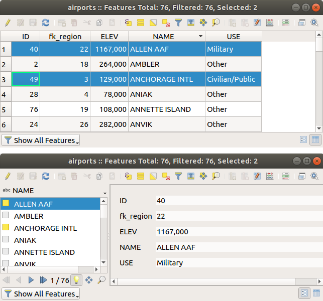
Fig. 12.74 Tabela de atributos na exibição de tabela (superior) vs exibição de formulário (inferior)
12.2.2.2. Configurando as colunas
Right-click in a column header when in table view to have access to tools that help you control:
Redimensionando larguras de colunas
A largura das colunas pode ser definida através de um clique com o botão direito do mouse no cabeçalho da coluna e selecione:
Defina a largura… para inserir o valor desejado. Por padrão, o valor atual é exibido no widget
Definir todas as larguras de coluna… para o mesmo valor
Autodimensionar para redimensionar da melhor forma possível a coluna.
Auto dimensionar todas as colunas
O tamanho de uma coluna também pode ser alterado arrastando o limite à direita de seu título. O novo tamanho da coluna é mantido para a camada e restaurado na próxima abertura da tabela de atributos.
In the Data Source Settings, you can choose to
 Autosize all columns by default when opening attribute table,
which will make “Autosize All Columns” the default view every time attribute tables are opened in QGIS.
Autosize all columns by default when opening attribute table,
which will make “Autosize All Columns” the default view every time attribute tables are opened in QGIS.
Ocultando e organizando colunas e permitindo ações
By right-clicking in a column header, you can choose to Hide column
from the attribute table (in “table view” mode).
For more advanced controls, press the  Organize columns…
button from the dialog toolbar or choose Organize columns…
in a column header contextual menu.
Organize columns…
button from the dialog toolbar or choose Organize columns…
in a column header contextual menu.
In the new dialog, you can:
check/uncheck columns you want to show or hide: a hidden column will disappear from every instance of the attribute table dialog until it is actively restored. It is also possible to:
choose Show All to display all the fields (columns) and actions in the table
choose Hide All to hide all the fields (columns) and actions in the table
use the Toggle selection to invert visibility of the current selection of columns. You can use keyboard combination for selecting multiple columns.
arraste e solte itens para reordenar as colunas na tabela de atributos. Observe que essa alteração é para a renderização da tabela e não altera a ordem dos campos na fonte de dados da camada
add a new virtual Actions column that displays in each row a drop-down box or a button list of enabled actions. See Propriedades de Ações for more information about actions.
Sorting rows
The rows can be sorted by any column, by clicking on the column header. A
small arrow indicates the sort order (downward pointing means descending
values from the top row down, upward pointing means ascending values from
the top row down).
You can also choose to sort the rows with the Sort… option of the
column header context menu and write an expression. E.g. to sort the rows
using multiple columns you can write concat(col0, col1).
Na exibição de formulário, o identificador de feições pode ser classificado usando o  :guilabel: opção Classificar por expressão de visualização.
Note that sorting the rows only affects the table rendering and does not alter the features order in the layer datasource.
Dica
Classificação com base em colunas de diferentes tipos
Trying to sort an attribute table based on columns of string and numeric types
may lead to unexpected result because of the concat("USE", "ID") expression
returning string values (ie, 'Borough105' < 'Borough6').
You can workaround this by using eg concat("USE", lpad("ID", 3, 0)) which
returns 'Borough105' > 'Borough006'.
12.2.2.3. Formatação de células da tabela usando condições
As configurações de formatação condicional podem ser usadas para realçar nas feições da tabela de atributos nos quais você deseja enfatizar, usando condições personalizadas nas feições:
geometria (por exemplo, identificando características de várias partes, áreas pequenas ou em uma extensão de mapa definida …);
or field value (e.g., comparing values to a threshold, identifying empty cells, duplicates, …).
You can enable the conditional formatting panel clicking on
 Conditional formatting button at the top right
of the attributes window in table view (not triggered in form view).
Conditional formatting button at the top right
of the attributes window in table view (not triggered in form view).
O novo painel permite que o usuário adicione novas regras para formatar a renderização de  Campo ou
  Linha completa. Adicionar nova regra abre um formulário para definir:
o nome da regra;
uma condição usando qualquer uma das funções construtor de expressões;
the formatting: it can be chosen from a list of predefined formats or created based on properties like:
cores de fundo e texto;
uso de ícone;
negrito, itálico, sublinhado ou strikeout;
fonte.
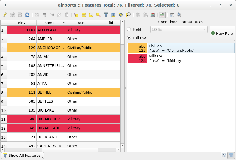
Fig. 12.75 Formatação condicional de uma tabela de atributo
12.2.3. Interagindo com feições em uma tabela de atributos
12.2.3.1. Selecionando características
Na exibição de tabela, cada linha da tabela de atributos exibe os atributos de um recurso exclusivo da camada. Selecionar uma linha seleciona o recurso e, da mesma forma, selecionar um recurso na tela do mapa (no caso de camada ativada para geometria) seleciona a linha na tabela de atributos. Se o conjunto de recursos selecionados na tela do mapa (ou tabela de atributos) for alterado, a seleção também será atualizada na tabela de atributos (ou tela do mapa) de acordo.
As linhas podem ser selecionadas clicando no número da linha no lado esquerdo da linha. Múltiplas linhas podem ser marcadas pressionando a tecla: kbd:Ctrl. Uma seleção contínua pode ser feita pressionando a tecla: kbd:Shift e clicando em vários cabeçalhos de linha no lado esquerdo das linhas. Todas as linhas entre a posição atual do cursor e a linha clicada são selecionadas. Mover a posição do cursor na tabela de atributos, clicando em uma célula na tabela, não altera a seleção de linha. Alterar a seleção na tela principal não move a posição do cursor na tabela de atributos.
Na exibição de formulário da tabela de atributos, as feições são identificados por padrão no painel esquerdo pelo valor do campo exibido (consulte: ref: maptips). Esse identificador pode ser substituído usando a lista suspensa na parte superior do painel, selecionando um campo existente ou usando uma expressão personalizada. Você também pode optar por classificar a lista de recursos no menu suspenso.
Clique em um valor no painel esquerdo para exibir os atributos da feição no caminho certo. Para selecionar uma feição, você precisa clicar dentro do símbolo quadrado à esquerda do identificador. Por padrão, o símbolo fica amarelo. Como na exibição de tabela, você pode executar várias seleções de recursos usando as combinações de teclado expostas anteriormente.
Beyond selecting features with the mouse, you can perform automatic selection based on feature’s attribute using tools available in the attribute table toolbar, such as (see section Seleção automática and subsequent for more information and use case):
 Selecione por expressão…
 Selecionar Feição pelo Valor…
 Desmarcar todas as feições da camada
 Selecionar Todas as Feições
 Inverter Feições Selecionadas.
It is also possible to select features using forms.
12.2.3.2. Filtragem de feições
Depois de selecionar as feições na tabela de atributos, você pode exibir apenas esses registros na tabela. Isso pode ser feito facilmente usando o item Mostrar feições selecionadas na lista suspensa no canto inferior esquerdo da caixa de diálogo da tabela de atributos. Esta lista oferece os seguintes filtros:
- Mostrar Todas as Feições
 Show Selected Features - same as using
Open Attribute Table (Selected Features) from the Layer
menu or the Attributes Toolbar or pressing Shift+F6
Show Selected Features - same as using
Open Attribute Table (Selected Features) from the Layer
menu or the Attributes Toolbar or pressing Shift+F6 Show Features visible on map - same as using
Open Attribute Table (Visible Features) from the Layer
menu or the Attributes Toolbar or pressing Ctrl+F6
Show Features visible on map - same as using
Open Attribute Table (Visible Features) from the Layer
menu or the Attributes Toolbar or pressing Ctrl+F6 Show Features with Failing Constraints -
features will be filtered to only show the ones which have failing constraints.
Depending on whether the unmet constraint is hard or soft,
failing field values are displayed in respectively dark or light orange cells.
Show Features with Failing Constraints -
features will be filtered to only show the ones which have failing constraints.
Depending on whether the unmet constraint is hard or soft,
failing field values are displayed in respectively dark or light orange cells. Show Edited and New Features - same as using
Open Attribute Table (Edited and New Features) from the Layer
menu or the Attributes Toolbar
Show Edited and New Features - same as using
Open Attribute Table (Edited and New Features) from the Layer
menu or the Attributes ToolbarField Filter - allows the user to filter based on value of a field: choose a column from a list, type or select a value and press Enter to filter. Then, only the features matching
num_field = valueorstring_field ilike '%value%'expression are shown in the attribute table. You can check
Case sensitive to be less permissive with strings. Advanced filter (Expression) - Opens the expression builder
dialog. Within it, you can create complex expressions to match table rows.
For example, you can filter the table using more than one field.
When applied, the filter expression will show up at the bottom of the form.
Advanced filter (Expression) - Opens the expression builder
dialog. Within it, you can create complex expressions to match table rows.
For example, you can filter the table using more than one field.
When applied, the filter expression will show up at the bottom of the form. : a shortcut to saved
expressions frequently used for filtering your attribute table.
: a shortcut to saved
expressions frequently used for filtering your attribute table.
Também é possível: ref: filtrar recursos usando formulários <filter_select_form>.
Nota
A filtragem de registros da tabela de atributos não filtra feições da camada; eles são simplesmente ocultados momentaneamente da tabela e podem ser acessados na tela do mapa ou removendo o filtro. Para filtros que ocultam recursos da camada, use o Query Builder.
Dica
Atualize a filtragem da fonte de dados com Mostrar feições visíveis no mapa
Quando, por motivos de desempenho, os recursos mostrados na tabela de atributos são espacialmente limitados à extensão da tela em sua abertura (consulte: ref: Opções da fonte de dados<tip_table_filtering> para obter instruções), selecionando: guilabel: Mostrar feições visíveis no mapa em um nova extensão de tela atualiza a restrição espacial.
12.2.3.3. Armazenamento de expressões de filtro
Expressions you use for attribute table filtering can be saved for further calls.
When using Field Filter or Advanced Filter (expression)
entries, the expression used is displayed in a text widget in the bottom of the
attribute table dialog. Press the  Save expression with text as name next to the box to save the expression
in the project. Pressing the drop-down menu next to the button allows to save
the expression with a custom name (Save expression as…).
Once a saved expression is displayed, the
button is triggered and its drop-down menu allows you to Edit the
expression and name if any, or Delete stored expression.
Save expression with text as name next to the box to save the expression
in the project. Pressing the drop-down menu next to the button allows to save
the expression with a custom name (Save expression as…).
Once a saved expression is displayed, the
button is triggered and its drop-down menu allows you to Edit the
expression and name if any, or Delete stored expression.
Saved filter expressions are saved in the project and available through the Stored filter expressions menu of the attribute table. They are different from the user expressions, shared by all projects of the active user profile.
12.2.3.4. Filtrando e selecionando feições usando formulários
Clicando no :sup: Filtre/selecione recursos usando o formulário ou pressione :kbd:Ctrl+F` fará com que a caixa de diálogo da tabela de atributos mude para a exibição do formulário e substitua cada widget por sua variante de pesquisa.
A partir deste ponto, a funcionalidade desta ferramenta é semelhante à descrita em: ref: select_by_value, onde é possível encontrar descrições de todos os operadores e selecionar modos.
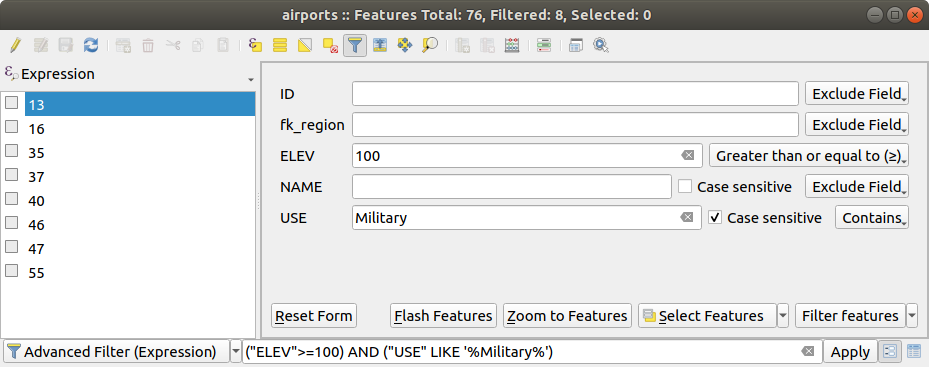
Fig. 12.76 Tabela de atributos filtrada pelo formulário de filtro
Ao selecionar / filtrar feições da tabela de atributos, existe um botão Filtro de feições que permite definir e refinar filtros. Seu uso aciona a opção: guilabel: Filtro avançado (Expressão) e exibe a expressão de filtro correspondente em um widget de texto editável na parte inferior do formulário.
Se já houver feições filtradas, você poderá refinar o filtro usando a lista suspensa ao lado do botão Filtro de feições. As opções são:
Filtrar dentro de (“AND”)
Estender filtro (“OR”)
Para limpar o filtro, selecione a opção Mostrar todas as feições no menu suspenso inferior esquerdo ou limpe a expressão e clique em Aplicar ou pressione Enter.
12.2.3.5. More actions on features
Users have several possibilities to manipulate feature in an attribute table. Right-click in a cell and you can:
Selecionar todas (Ctrl+A) as feições;
Copie o conteúdo de uma célula na área de transferência com: guilabel:Copiar conteúdo da célula;
Aproximar na feição sem ter que selecioná-lo previamente;
Panorâmica da feição sem ter que selecioná-lo previamente;
Destacar feição, para destacá-la na tela do mapa;
Abrir formulário: alterna a tabela de atributos para a exibição de formulários, com foco na feição clicado.
Display a list of actions, previously enabled in the tab.
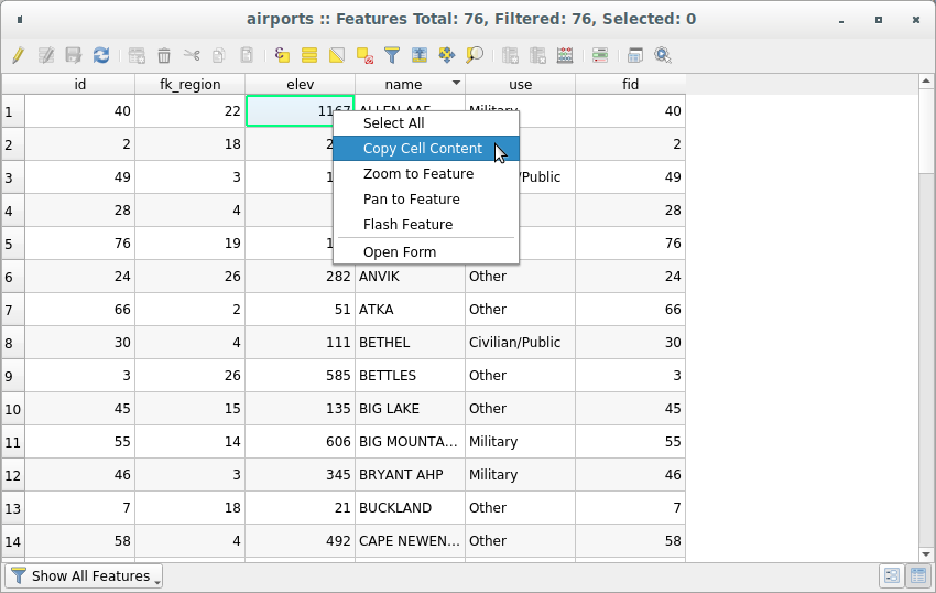
Fig. 12.77 Copiar botão de conteúdo da célula
If you want to use attribute data in external programs (such as Excel,
LibreOffice, or a custom web application), select one or more row(s) and
use the  Copy selected rows to clipboard button
or press Ctrl+C.
Moreover, in menu
you can define the format to paste to with the Copy features as option.
More details at Configurações de fonte de informação.
Copy selected rows to clipboard button
or press Ctrl+C.
Moreover, in menu
you can define the format to paste to with the Copy features as option.
More details at Configurações de fonte de informação.
12.2.4. Editando valores de atributo
In order to modify data in an attribute table, you should first toggle the layer into edit.
Press the  Toggle Editing button.
Depending on the layer geometry type and the clipboard state,
a few more tools are enabled in the attribute table top toolbar.
Toggle Editing button.
Depending on the layer geometry type and the clipboard state,
a few more tools are enabled in the attribute table top toolbar.
Editing attribute values can then be done by:
digitando o novo valor diretamente na célula, esteja a tabela de atributos na visualização de tabela ou formulário. As mudanças são feitas célula por célula, feição por feição;
using the field calculator: update in a row a field that may already exist or to be created but for multiple features. It can be used to create virtual fields;
using the quick field calculation bar: same as above but for only existing field;
or using the multi edit mode: update in a row multiple fields for multiple features.
Putting the layer into edit mode will also allow you to
 Paste features from clipboard (Ctrl+V)
 Cut selected rows to clipboard (Ctrl+X)
or
Cut selected rows to clipboard (Ctrl+X)
or  Delete selected features.
More details at Cortando, Copiando e Colando Elementos.
Delete selected features.
More details at Cortando, Copiando e Colando Elementos.
12.2.4.1. Utilizando a Calculadora de Campo
The  Field Calculator button in the attribute table
allows you to perform calculations on the basis of existing attribute values or
defined functions, for instance, to calculate length or area of geometry features.
The results can be used to update an existing field, or written
to a new field (that can be a virtual one).
Field Calculator button in the attribute table
allows you to perform calculations on the basis of existing attribute values or
defined functions, for instance, to calculate length or area of geometry features.
The results can be used to update an existing field, or written
to a new field (that can be a virtual one).
The field calculator is available on any layer that supports edit. When you click on the field calculator icon the dialog opens (see Fig. 12.78). If the layer is not in edit mode, a warning is displayed and using the field calculator will cause the layer to be put in edit mode before the calculation is made.
Based on the Expression Builder dialog, the field calculator dialog offers a complete interface to define an expression and apply it to an existing or a newly created field. To use the field calculator dialog, you must select whether you want to:
aplicar o cálculo sobre toda a camada ou apenas sobre as características selecionadas
criar um novo campo para o cálculo ou atualizar um já existente.
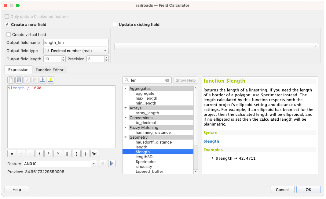
Fig. 12.78 Calculadora de campo
If you choose to add a new field, you need to enter a field name, a field type (integer, real, date or string) and if needed, the total field length and the field precision. For example, if you choose a field length of 10 and a field precision of 3, it means you have 7 digits before the dot, and 3 digits for the decimal part.
A short example illustrates how field calculator works when using the
Expression tab. We want to calculate the length in km of the
railroads layer from the QGIS sample dataset:
Load the shapefile
railroads.shpin QGIS and press
Open Attribute Table.Click on
Toggle editing mode and open the
Field Calculator dialog.Select the
Create a new field checkbox to save the
calculations into a new field.Set Output field name to
length_kmSelecione
Número decimal (real)como Tipo de campo de saída`.Set the Output field length to
10and the Precision to3Double click on
$lengthin the Geometry group to add the length of the geometry into the Field calculator expression box (you will begin to see a preview of the output, up to 60 characters, below the expression box updating in real-time as the expression is assembled).Complete the expression by typing
/ 1000in the Field calculator expression box and click OK.You can now find a new length_km field in the attribute table.
12.2.4.2. Criando um campo virtual
A virtual field is a field based on an expression calculated on the fly, meaning
that its value is automatically updated as soon as an underlying parameter changes.
The expression applies to all the features in the layer and is set once;
you no longer need to recalculate the field each time underlying values change.
For example, you may want to use a virtual field if you need area to be evaluated
as you digitize features or to automatically calculate a duration between dates
that may change (e.g., using now() function).
Creating a virtual field is done through the Field calculator dialog
and follows the same procedure as for regular fields.
Simply remember to check the Create virtual field option
and use a field type compatible with the data your expression would generate.
Editing a virtual field is done through the  Fields tab
of the layer properties dialog (see Propriedades dos campos).
The expression defining the field is exposed in the Comment column,
and pressing the
Fields tab
of the layer properties dialog (see Propriedades dos campos).
The expression defining the field is exposed in the Comment column,
and pressing the  button next to it opens an expression editor window
for update.
button next to it opens an expression editor window
for update.
Nota
Uso de campos virtuais
A field can be set virtual only at its creation.
Os campos virtuais não são permanentes nos atributos da camada, o que significa que eles são salvos e disponibilizados apenas no arquivo de projeto em que foram criados.
12.2.4.3. Usando a barra de cálculo rápido de campo
While Field calculator is always available, the quick field calculation bar on top of the attribute table is only visible if the layer is in edit mode. Thanks to the expression engine, it offers a quicker access to edit an already existing field:
Selecione o campo a ser atualizado na lista suspensa.
Fill the textbox with a value, an expression you directly write or build using the
expression button.Click on Update All, Update Selected or Update Filtered button according to your need.
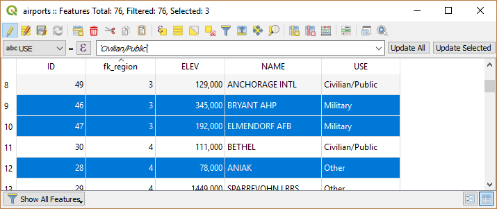
Fig. 12.79 Barra de cálculo rápido de campo
12.2.4.4. Editando vários campos
Ao contrário das ferramentas anteriores, o modo de edição múltipla permite que vários atributos de diferentes recursos sejam editados simultaneamente. Quando a camada é alternada para edição, os recursos de edição múltipla ficam acessíveis:
using the
 Toggle multi edit mode button from the toolbar
inside the attribute table dialog;
Toggle multi edit mode button from the toolbar
inside the attribute table dialog;or selecting
menu.
Nota
Unlike the tool from the attribute table, hitting the option provides you with a modal dialog to fill attributes changes. Hence, features selection is required before execution.
Para editar vários campos em uma linha:
Selecione as feições que você deseja editar.
From the attribute table toolbar, click the
button. This will
toggle the dialog to its form view. Feature selection could also be made
at this step.At the right side of the attribute table, fields (and values) of selected features are shown. New widgets appear next to each field allowing for display of the current multi edit state:
 The field contains different values for selected
features. It’s shown empty and each feature will keep its original value.
You can reset the value of the field from the drop-down list of the widget.
The field contains different values for selected
features. It’s shown empty and each feature will keep its original value.
You can reset the value of the field from the drop-down list of the widget. All selected features have the same value for this
field and the value displayed in the form will be kept.
All selected features have the same value for this
field and the value displayed in the form will be kept. The field has been edited and the entered value
will be applied to all the selected features. A message appears at the top
of the dialog, inviting you to either apply or reset your modification.
The field has been edited and the entered value
will be applied to all the selected features. A message appears at the top
of the dialog, inviting you to either apply or reset your modification.
Clicking any of these widgets allows you to either set the current value for the field or reset to original value, meaning that you can roll back changes on a field-by-field basis.
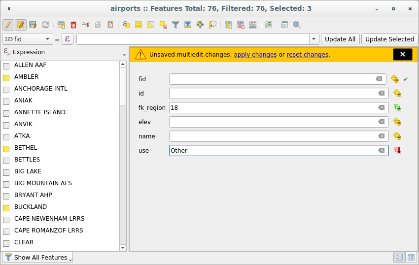
Fig. 12.80 Campos de edição de múltiplas feições
Faça as alterações nos campos desejados.
Clique em Aplicar alterações no texto da mensagem superior ou em qualquer outro recurso no painel esquerdo.
As alterações serão aplicadas a todos os recursos selecionados. Se nenhum recurso for selecionado, toda a tabela será atualizada com suas alterações. As modificações são feitas como um único comando de edição. Então, pressionando |desfazer| Desfazer reverterá as alterações de atributo para todos os recursos selecionados de uma só vez.
Nota
O modo de edição múltipla só está disponível para formulários gerados automaticamente e de arrastar e soltar (veja personalizar_formulário); ele não é suportado por formulários de interface do usuário personalizados.
12.2.5. Exploring features attributes through the Identify Tool
The  Identify features tool can be used to display all attributes
of a feature in the map canvas. It is a quick way to view and verify all data without
having to search for it in the attribute table.
Identify features tool can be used to display all attributes
of a feature in the map canvas. It is a quick way to view and verify all data without
having to search for it in the attribute table.
To use the Identify features tool for vector layers, follow these steps:
Select the vector layer in the Layers panel.
Click on the Identify features tool in the toolbar or press Ctrl+Shift+I.
Click on a feature in the map view.
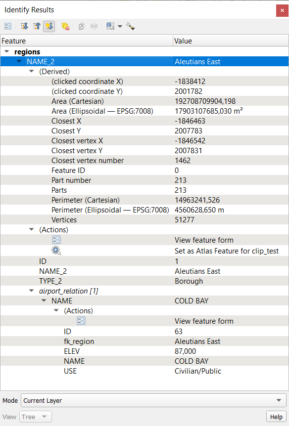
Fig. 12.81 Identify Results dialog
The Identify results panel will display different features information in a tree view. There are two columns in the panel: Feature and Value. The first item is the name of the layer and its children are its identified feature(s). Each feature is identified by the display name field along with its value. Other information about the feature follows:
Derived section - those are the information calculated or derived from other information in the layer. For example, the area of a polygon or the length of a line. General information that can be found in this section:
Depending on the geometry type, the cartesian measurements of length, perimeter or area in the layer’s CRS units. For 3D line vectors, the cartesian line length is available.
Depending on the geometry type and if an ellipsoid is set in the Project Properties dialog (), ellipsoidal values of length, perimeter, or area using the specified units.
The count of geometry parts in the feature and the number of the part clicked.
The count of vertices in the feature.
Coordinate information, using the project properties Coordinates display settings:
XandYcoordinate values of the clicked pointthe number of the closest vertex to the clicked point
Valores de coordenadas
XeYdo vértice mais próximo (eZ/Mse aplicável)se você clicar em um segmento curvo, o raio dessa seção também será mostrado.
if both the vector layer and the project have vertical datums set and they differ, the
Zvalue will be displayed for both datums.
Actions: Actions can be added to the identify feature windows. The action is run by clicking on the action label. By default, only one action is added, namely
View feature formfor editing. You can define more actions in the layer’s properties dialog (see Propriedades de Ações).Data attributes: This is the list of attribute fields and values for the feature that has been clicked.
Nota
Links in the feature’s attributes are clickable from the Identify Results panel and will open in your default web browser.
When a vector layer has defined relations, the Identify Results panel can display both referenced and referencing related features. To view these relations, ensure that the Show relations option is enabled in the Identify Settings. Available information for each related feature include:
the name of the relation and the linked layer
the entry in the referenced or referencing field, identifying the feature
the activated actions
the list of attribute fields and values
You can expand related features to explore connected records through multiple levels, including many-to-many (n:m) and polymorphic relations. Only nodes you explicitly expand are loaded, preventing excessive nesting.
To focus on a specific related record, right-click it and choose Identify Feature. This re-centers the identify results on the selected feature, starting a new identification tree from it and effectively limiting the visible nesting depth. Features already shown in ancestor nodes are automatically omitted to avoid duplicates or circular relations.