8.3. Lesson: 지형 분석
래스터가 표현하고 있는 지형에 대해 더 깊이 이해할 수 있게 해주는 특정한 래스터 형식이 있습니다. 수치 표고 모델(DEM)이 이런 점에서 특히 유용합니다. 이 강의에서는 지형 분석을 이용해서, 이전 모듈에서 다뤘던 주거 구역 개발에 대해 더 자세히 알아보도록 하겠습니다.
이 강의의 목표: 지형 분석을 이용해서 지형에 대해 더 많은 정보를 끌어내기.
8.3.1.  Follow Along: 음영기복도 계산
The DEM you have on your map right now does show you the elevation of the terrain, but it can sometimes seem a little abstract. It contains all the 3D information about the terrain that you need, but it doesn’t look like a 3D object. To get a better look at the terrain, it is possible to calculate a hillshade, which is a raster that maps the terrain using light and shadow to create a 3D-looking image.
To work with DEMs, you should use QGIS’ all-in-one DEM (Terrain models) analysis tool.
- Click on the menu item Raster ‣ Analysis ‣ DEM (Terrain models).
- In the dialog that appears, ensure that the Input file is the DEM layer.
- Set the Output file to hillshade.tif in the directory exercise_data/residential_development.
- Also make sure that the Mode option has Hillshade selected.
- Check the box next to Load into canvas when finished.
- You may leave all the other options unchanged.
- Click OK to generate the hillshade.
- When it tells you that processing is completed, click OK on the message to get rid of it.
- Click Close on the main DEM (Terrain models) dialog.
이제 다음과 같이 hillshade 라는 새 레이어가 생성되었습니다.
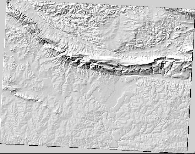
멋진 3D로 보입니다만, 좀 더 향상시킬 수 있을까요? 음영기복도 그 자체로는 마치 석고 모형처럼 보입니다. 다른, 좀 더 다채로운 래스터들과 어떻게 함께 사용할 수는 없을까요? 물론 할 수 있습니다. 음영기복도를 오버레이로서 사용한다면 말이죠.
8.3.2. Follow Along: 음영기복도를 오버레이로 사용
음영기복도는 낮 동안의 특정 시간의 햇빛에 대한 유용한 정보를 제공할 수 있습니다. 하지만 맵을 더 보기 좋게 하기 위한 심미적 목적을 위해서도 사용할 수 있습니다. 이렇게 하려면 음영기복도를 거의 투명하게 설정하면 됩니다.
Change the symbology of the original DEM to use the Pseudocolor scheme as in the previous exercise.
Hide all the layers except the DEM and hillshade layers.
Click and drag the DEM to be beneath the hillshade layer in the Layers list.
Set the hillshade layer to be transparent by opening its Layer Properties and go to the Transparency tab.
Set the Global transparency to 50%:
Click OK on the Layer Properties dialog. You’ll get a result like this:
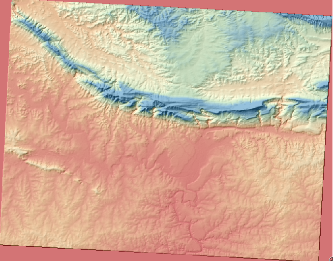
Switch the hillshade layer off and back on in the Layers list to see the difference it makes.
음영기복도를 이런 식으로 사용하면 경관의 지형을 향상시킬 수 있습니다. 만약 그 효과가 미미하다고 느껴진다면, hillshade 레이어의 투명도를 조절할 수 있습니다. 하지만 물론, 음영기복도가 밝아질수록 그 아래의 색상은 침침해질 것입니다. 여러분이 만족할 수 있는 균형을 찾아야 합니다.
Remember to save your map when you are done.
주석
For the next two exercises, please use a new map. Load only the DEM raster dataset into it (exercise_data/raster/SRTM/srtm_41_19.tif). This is to simplify matters while you’re working with the raster analysis tools. Save the map as exercise_data/raster_analysis.qgs.
8.3.3.  Follow Along: 경사도 계산
지형에 대해 알아두면 좋은 점 가운데 하나는 얼마나 가파르냐는 것입니다. 예를 들어 어떤 토지에 집을 짓고 싶다고 할 때, 그 토지는 어느 정도 평평해야 할 것입니다.
To do this, you need to use the Slope mode of the DEM (Terrain models) tool.
Open the tool as before.
Select the Mode option Slope:
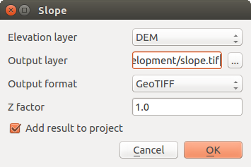
Set the save location to exercise_data/residential_development/slope.tif
Enable the Load into canvas... checkbox.
Click OK and close the dialogs when processing is complete, and click Close to close the dialog. You’ll see a new raster loaded into your map.
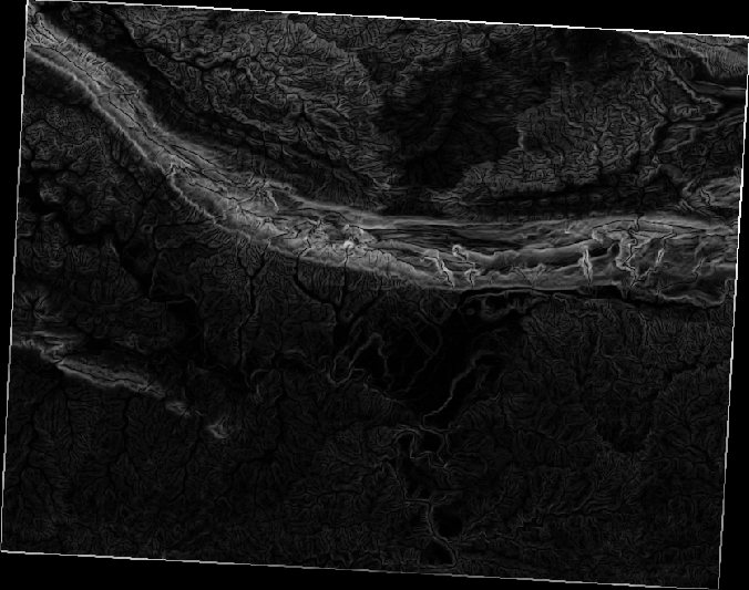
With the new raster selected in the Layers list, click the Stretch Histogram to Full Dataset button. Now you’ll see the slope of the terrain, with black pixels being flat terrain and white pixels, steep terrain:
8.3.4. Try Yourself calculating the aspect
The aspect of terrain refers to the direction it’s facing in. Since this study is taking place in the Southern Hemisphere, properties should ideally be built on a north-facing slope so that they can remain in the sunlight.
- Use the Aspect mode of the DEM (Terain models) tool to calculate the aspect of the terrain.
8.3.5. Follow Along: 래스터 계산기 사용
벡터 분석 강의에서 마지막으로 다뤘던 부동산 중개업자 문제를 다시 떠올려보십시오. 그때의 구매자가 지금은 건물을 산 다음 부지 내에 작은 집을 짓고 싶어 한다고 해봅시다. 남반구에서 이런 개발에 이상적인 계획은 우선 5˚ 미만 경사의 북쪽을 면한 토지가 있어야 할 것입니다. 그러나 경사가 2˚ 미만인 경우, 향은 문제가 되지 않습니다.
다행히 여러분에게는 이미 경사는 물론 향을 보여주는 래스터가 있습니다. 그런데 이 두 가지 조건을 동시에 만족하는 곳을 알 도리가 없죠. 어떻게 이런 분석을 할 수 있을까요?
그 답은 Raster calculator 가 가지고 있습니다.
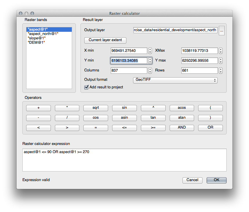
- Click on Raster > Raster calculator... to start this tool.
- To make use of the aspect dataset, double-click on the item aspect@1 in the Raster bands list on the left. It will appear in the Raster calculator expression text field below.
North is at 0 (zero) degrees, so for the terrain to face north, its aspect needs to be greater than 270 degrees and less than 90 degrees.
In the Raster calculator expression field, enter this expression:
aspect@1 <= 90 OR aspect@1 >= 270
Set the output file to aspect_north.tif in the directory exercise_data/residential_development/.
Ensure that the box Add result to project is checked.
Click OK to begin processing.
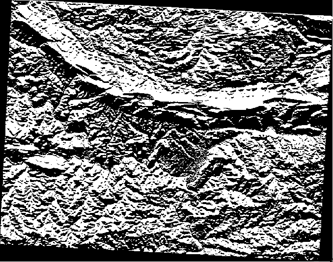
결과는 다음과 같을 것입니다.
8.3.6. Try Yourself
이제 향 작업을 끝냈으니, DEM 레이어에 대한 두 가지 새로운 분석을 생성해봅시다.
- The first will be to identify all areas where the slope is less than or equal to 2 degrees.
- The second is similar, but the slope should be less than or equal to 5 degrees.
- Save them under exercise_data/residential_development/ as slope_lte2.tif and slope_lte5.tif.
8.3.7. Follow Along: 래스터 분석 결과 결합
이제 다음과 같은 DEM 레이어의 세 가지 분석 래스터가 생겼습니다.
aspect_north : 북쪽을 면한 지형
slope_lte2: 경사가 2˚ 이하인 지형
slope_lte5: 경사가 5˚ 이하인 지형
Where the conditions of these layers are met, they are equal to 1. Elsewhere, they are equal to 0. Therefore, if you multiply one of these rasters by another one, you will get the areas where both of them are equal to 1.
만족해야 하는 조건은 다음과 같습니다. 경사가 5˚ 이하이며, 북쪽을 면하는 지형일 것, 다만 경사가 2˚ 이하인 곳은 해당 지형이 어느쪽을 면하든지 상관 없슴.
Therefore, you need to find areas where the slope is at or below 5 degrees AND the terrain is facing north; OR the slope is at or below 2 degrees. Such terrain would be suitable for development.
이 기준들을 만족하는 지역을 계산하려면,
Open your Raster calculator again.
Use the Raster bands list, the Operators buttons, and your keyboard to build this expression in the Raster calculator expression text area:
( aspect_north@1 = 1 AND slope_lte5@1 = 1 ) OR slope_lte2@1 = 1
Save the output under exercise_data/residential_development/ as all_conditions.tif.
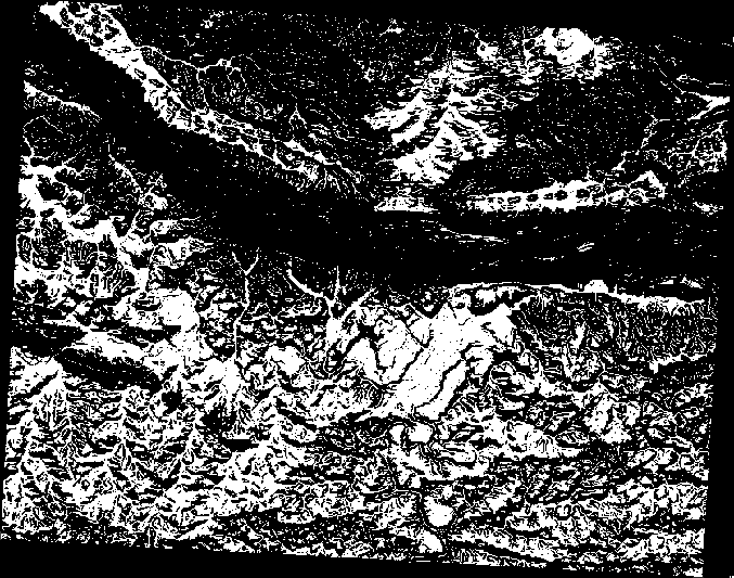
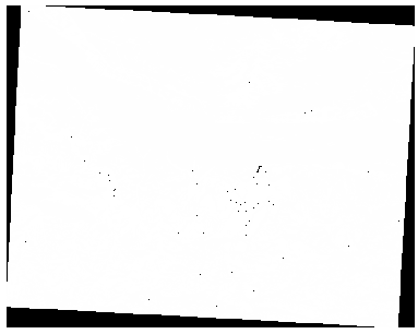
Click OK on the Raster calculator. Your results:
8.3.8. Follow Along: 래스터 단순화
앞의 이미지에서 볼 수 있듯이, 이렇게 결합된 분석의 결과물은 조건을 만족하는 수많은, 아주 작은 지역들로 이루어져 있습니다. 그러나 이 결과는 우리의 분석에 그다지 쓸모가 없습니다. 뭔가를 짓기에는 너무 작은 토지들이니까요. 이 쓸모 없는 작은 토지들을 제거해보겠습니다.
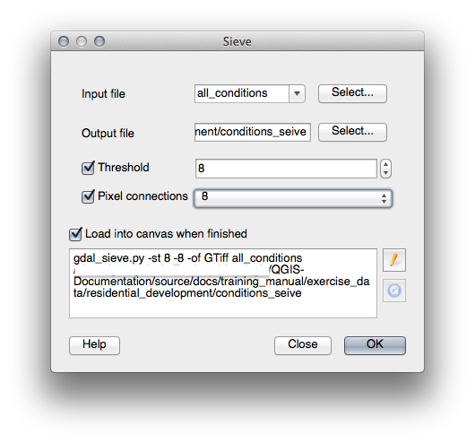
- Open the Sieve tool (Raster ‣ Analysis ‣ Sieve).
- Set the Input file to all_conditions, and the Output file to all_conditions_sieve.tif (under exercise_data/residential_development/).
- Set both the Threshold and Pixel connections values to 8, then run the tool.
Once processing is done, the new layer will load into the canvas. But when you try to use the histogram stretch tool to view the data, this happens:
무엇 때문일까요? 그 답은 이 새 래스터 파일의 메타데이터에 있습니다.
- View the metadata under the Metadata tab of the Layer Properties dialog. Look in the Properties section at the bottom.
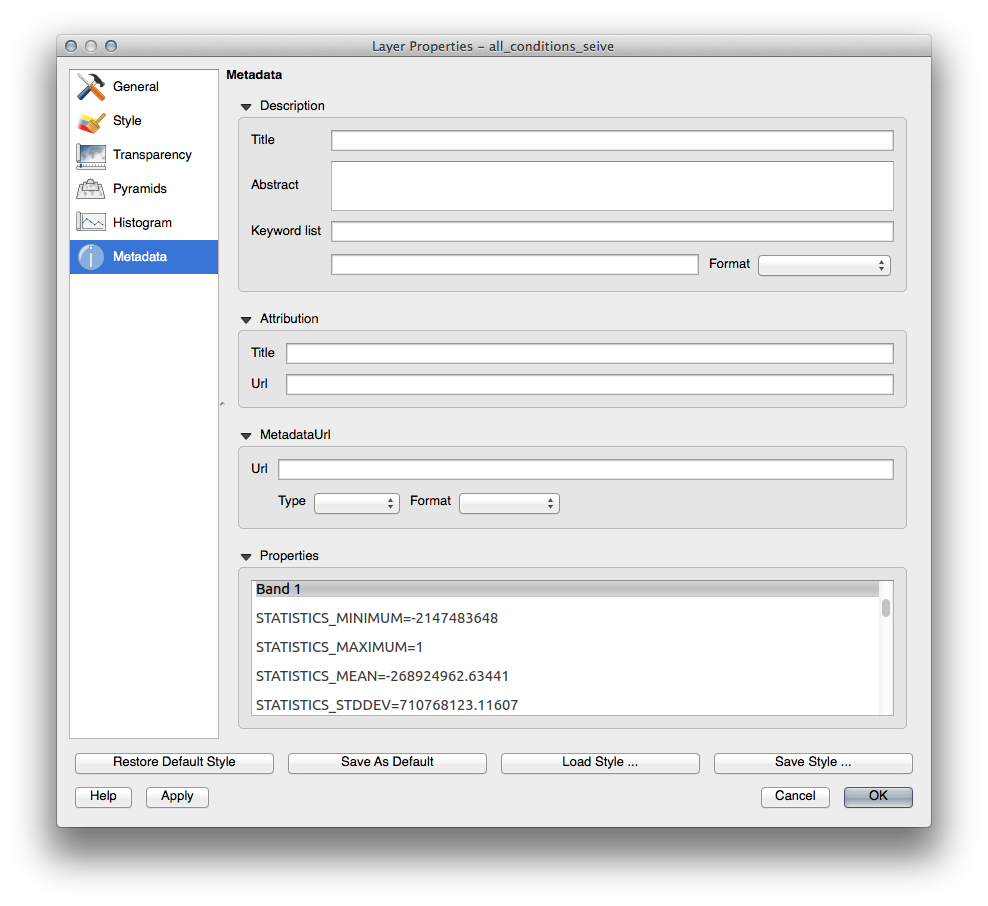
Whereas this raster, like the one it’s derived from, should only feature the values 1 and 0, it has the STATISTICS_MINIMUM value of a very large negative number. Investigation of the data shows that this number acts as a null value. Since we’re only after areas that weren’t filtered out, let’s set these null values to zero.
Open the Raster Calculator again, and build this expression:
(all_conditions_sieve@1 <= 0) = 0
This will maintain all existing zero values, while also setting the negative numbers to zero; which will leave all the areas with value 1 intact.
Save the output under exercise_data/residential_development/ as all_conditions_simple.tif.
산출물은 다음과 같습니다.
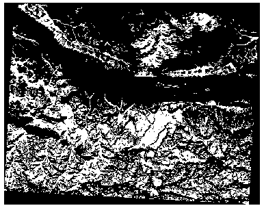
우리가 기대한 산출물입니다. 이전 결과물을 단순화시킨 버전이죠. 어떤 도구의 결과물이 기대했던 것과 다를 경우, 문제를 해결 하는 데 메타데이터(및, 적용 가능할 경우 벡터 속성)을 살펴보는 작업이 필수적일 수도 있습니다.
8.3.9. In Conclusion
You’ve seen how to derive all kinds of analysis products from a DEM. These include hillshade, slope and aspect calculations. You’ve also seen how to use the raster calculator to further analyze and combine these results.
8.3.10. What’s Next?
이제 여러분은 두 가지 분석을 할 수 있습니다. 벡터 분석은 잠재적으로 적합한 계획을 보여주며, 래스터 분석은 잠재적으로 적합한 지형을 보여줍니다. 이들을 어떻게 결합해야 문제에 대한 최종 결론을 얻을 수 있을까요? 이것이 다음 모듈에서 시작하는 강의의 주제입니다.