Important
Traducerea este un efort al comunității, la care puteți să vă alăturați. În prezent, această pagină este tradusă 7.38%.
23.11. Configurarea Aplicațiilor Externe
The Processing framework can be extended using additional applications. Algorithms that rely on external applications are managed by their own algorithm providers. Additional providers can be found as separate plugins, and installed using the QGIS Plugin Manager.
This section will show you how to configure the Processing framework to include these additional applications, and it will explain some particular features of the algorithms based on them. Once you have correctly configured the system, you will be able to execute external algorithms from any component like the toolbox or the model designer, just like you do with any other algorithm.
By default, algorithms that rely on an external application not shipped with QGIS are not enabled. You can enable them in the Processing settings dialog if they are installed on your system.
23.11.1. O notă pentru utilizatorii de Windows
If you are not an advanced user and you are running QGIS on Windows, you might not be interested in reading the rest of this chapter. Make sure you install QGIS in your system using the standalone installer. That will automatically install GRASS in your system and configure it so it can be run from QGIS. All the algorithms from this provider will be ready to be run without needing any further configuration. If installing with the OSGeo4W application, make sure that you also select GRASS for installation.
23.11.2. O notă privind formatele de fișiere
When using external software, opening a file in QGIS does not mean that it can be opened and processed in that other software. In most cases, other software can read what you have opened in QGIS, but in some cases, that might not be true. When using databases or uncommon file formats, whether for raster or vector layers, problems might arise. If that happens, try to use well-known file formats that you are sure are understood by both programs, and check the console output (in the log panel) to find out what is going wrong.
You might for instance get trouble and not be able to complete your work if you call an external algorithm with a GRASS raster layers as input. For this reason, such layers will not appear as available to algorithms.
You should, however, not have problems with vector layers, since QGIS automatically converts from the original file format to one accepted by the external application before passing the layer to it. This adds extra processing time, which might be significant for large layers, so do not be surprised if it takes more time to process a layer from a DB connection than a layer from a Shapefile format dataset of similar size.
Providers not using external applications can process any layer that you can open in QGIS, since they open it for analysis through QGIS.
All raster and vector output formats produced by QGIS can be used as input layers. Some providers do not support certain formats, but all can export to common formats that can later be transformed by QGIS automatically. As for input layers, if a conversion is needed, that might increase the processing time.
23.11.3. O notă privind selecțiile stratului vectorial
External applications may also be made aware of the selections that exist in vector layers within QGIS. However, that requires rewriting all input vector layers, just as if they were originally in a format not supported by the external application. Only when no selection exists, or the Use only selected features option is not enabled in the processing general configuration, can a layer be directly passed to an external application.
In other cases, exporting only selected features is needed, which causes longer execution times.
23.11.4. Using third-party Providers
23.11.4.1. R scripts and libraries
To enable R in Processing you need to install the Processing R Provider plugin and configure R for QGIS.
Configuration is done in in the Processing tab of .
Depending on your operating system, you may have to use R folder to specify where your R binaries are located.
Notă
On Windows the R executable file is normally in
a folder (R-<version>) under C:\Program Files\R\.
Specify the folder and NOT the binary!
On Linux you just have to make sure that the R folder is
in the PATH environment variable.
If R in a terminal window starts R, then you are ready to go.
After installing the Processing R Provider plugin, you will find some example scripts in the Processing Toolbox:
Scatterplot runs an R function that produces a scatter plot from two numerical fields of the provided vector layer.
test_sf does some operations that depend on the
sfpackage and can be used to check if the R packagesfis installed. If the package is not installed, R will try to install it (and all the packages it depends on) for you, using the Package repository specified in in the Processing options. The default is https://cran.r-project.org/. Installing may take some time…test_sp can be used to check if the R package
spis installed. If the package is not installed, R will try to install it for you.
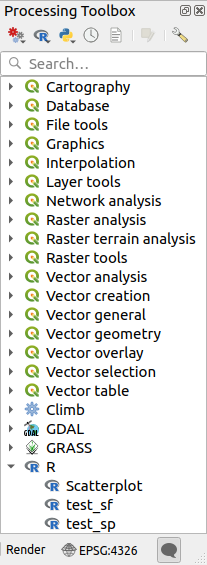
If you have R configured correctly for QGIS, you should be able to run these scripts.
Adding R scripts from the QGIS collection
R integration in QGIS is different from that of some other third party providers like SAGA in that there is not a predefined set of algorithms you can run (except for some example script that come with the Processing R Provider plugin).
A set of example R scripts is available in the QGIS Repository. Perform the following steps to load and enable them using the QGIS Resource Sharing plugin.
Add the QGIS Resource Sharing plugin (you may have to enable Show also experimental plugins in the Plugin Manager Settings)
Open it ()
Choose the Settings tab
Click Reload repositories
Choose the All tab
Select QGIS R script collection in the list and click on the Install button
The collection should now be listed in the Installed tab
Close the plugin
Open the Processing Toolbox, and if everything is OK, the example scripts will be present under R, in various groups (only some of the groups are expanded in the screenshot below).
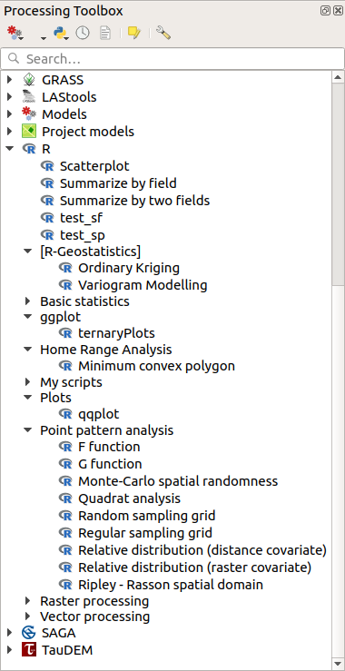
Fig. 23.35 The Processing Toolbox with some R scripts shown
The scripts at the top are the example scripts from the Processing R Provider plugin.
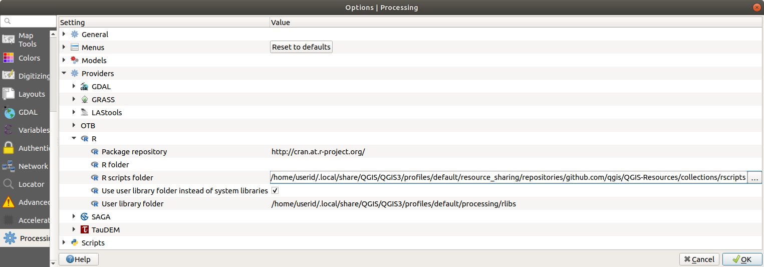
If, for some reason, the scripts are not available in the Processing Toolbox, you can try to:
Open the Processing settings ( tab)
Go to
On Ubuntu, set the path to (or, better, include in the path):
/home/<user>/.local/share/QGIS/QGIS3/profiles/default/resource_sharing/repositories/github.com/qgis/QGIS-Resources/collections/rscripts
On Windows, set the path to (or, better, include in the path):
C:\Users\<user>\AppData\Roaming\QGIS\QGIS3\profiles\default\resource_sharing\repositories\github.com\qgis\QGIS-Resources\collections\rscripts
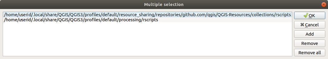
To edit, double-click. You can then choose to just paste / type the path, or you can navigate to the directory by using the … button and press the Add button in the dialog that opens. It is possible to provide several directories here. They will be separated by a semicolon („;”).
If you would like to get all the R scripts from the QGIS 2 on-line collection, you can select QGIS R script collection (from QGIS 2) instead of QGIS R script collection. You will probably find that scripts that depend on vector data input or output will not work.
Creating R scripts
You can write scripts and call R commands, as you would do from R. This section shows you the syntax for using R commands in QGIS, and how to use QGIS objects (layers, tables) in them.
To add an algorithm that calls an R function (or a more complex R script that you have developed and you would like to have available from QGIS), you have to create a script file that performs the R commands.
R script files have the extension .rsx, and creating them is
pretty easy if you just have a basic knowledge of R syntax and R
scripting.
They should be stored in the R scripts folder.
You can specify the folder (R scripts folder) in the
R settings group in Processing settings dialog).
Let’s have a look at a very simple script file, which calls the R
method spsample to create a random grid within the boundary of the
polygons in a given polygon layer.
This method belongs to the maptools package.
Since almost all the algorithms that you might like to incorporate
into QGIS will use or generate spatial data, knowledge of spatial
packages like maptools and sp/sf, is very useful.
##Random points within layer extent=name
##Point pattern analysis=group
##Vector_layer=vector
##Number_of_points=number 10
##Output=output vector
library(sp)
spatpoly = as(Vector_layer, "Spatial")
pts=spsample(spatpoly,Number_of_points,type="random")
spdf=SpatialPointsDataFrame(pts, as.data.frame(pts))
Output=st_as_sf(spdf)
The first lines, which start with a double Python comment sign
(##), define the display name and group of the script, and
tell QGIS about its inputs and outputs.
Notă
To find out more about how to write your own R scripts, have a look at the R Intro section in the training manual and consult the QGIS R Syntax section.
When you declare an input parameter, QGIS uses that information for two things: creating the user interface to ask the user for the value of that parameter, and creating a corresponding R variable that can be used as R function input.
In the above example, we have declared an input of type vector,
named Vector_layer.
When executing the algorithm, QGIS will open the layer selected
by the user and store it in a variable named Vector_layer.
So, the name of a parameter is the name of the variable that you
use in R for accessing the value of that parameter (you should
therefore avoid using reserved R words as parameter names).
Spatial parameters such as vector and raster layers are read using
the st_read() (or readOGR) and brick() (or readGDAL)
commands (you do not have to worry about adding those commands to
your description file – QGIS will do it), and they are stored as
sf (or Spatial*DataFrame) objects.
Table fields are stored as strings containing the name of the selected field.
Vector files can be read using the readOGR() command instead
of st_read() by specifying ##load_vector_using_rgdal.
This will produce a Spatial*DataFrame object instead of an
sf object.
Raster files can be read using the readGDAL() command instead
of brick() by specifying ##load_raster_using_rgdal.
If you are an advanced user and do not want QGIS to create the
object for the layer, you can use ##pass_filenames to indicate
that you prefer a string with the filename.
In this case, it is up to you to open the file before performing
any operation on the data it contains.
With the above information, it is possible to understand the first lines of the R script (the first line not starting with a Python comment character).
library(sp)
spatpoly = as(Vector_layer, "Spatial")
pts=spsample(polyg,numpoints,type="random")
The spsample function is provided by the sp library, so
the first thing we do is to load that library.
The variable Vector_layer contains an sf object.
Since we are going to use a function (spsample) from the sp
library, we must convert the sf object to a
SpatialPolygonsDataFrame object using the as function.
Then we call the spsample function with this object and
the numpoints input parameter (which specifies the number of
points to generate).
Since we have declared a vector output named Output, we have to
create a variable named Output containing an sf object.
We do this in two steps.
First we create a SpatialPolygonsDataFrame object from the
result of the function, using the SpatialPointsDataFrame function,
and then we convert that object to an sf object using the
st_as_sf function (of the sf library).
You can use whatever names you like for your intermediate
variables.
Just make sure that the variable storing your final result has
the defined name (in this case Output), and that it contains
a suitable value (an sf object for vector layer output).
In this case, the result obtained from the spsample method had
to be converted explicitly into an sf object via a
SpatialPointsDataFrame object, since it is itself an object of
class ppp, which can not be returned to QGIS.
If your algorithm generates raster layers, the way they are saved
will depend on whether or not you have used the
##dontuserasterpackage option.
If you have used it, layers are saved using the writeGDAL()
method.
If not, the writeRaster() method from the raster package
will be used.
If you have used the ##pass_filenames option, outputs are
generated using the raster package (with writeRaster()).
If your algorithm does not generate a layer, but a text result in
the console instead, you have to indicate that you want the
console to be shown once the execution is finished.
To do so, just start the command lines that produce the results
you want to print with the > («greater than») sign.
Only output from lines prefixed with > are shown.
For instance, here is the description file of an algorithm that
performs a normality test on a given field (column) of the
attributes of a vector layer:
##layer=vector
##field=field layer
##nortest=group
library(nortest)
>lillie.test(layer[[field]])
The output of the last line is printed, but the output of the first is not (and neither are the outputs from other command lines added automatically by QGIS).
If your algorithm creates any kind of graphics (using the plot()
method), add the following line (output_plots_to_html used to be
showplots):
##output_plots_to_html
This will cause QGIS to redirect all R graphical outputs to a temporary file, which will be opened once R execution has finished.
Both graphics and console results will be available through the processing results manager.
For more information, please check the R scripts in the official QGIS collection (you download and install them using the QGIS Resource Sharing plugin, as explained in Adding R scripts from the QGIS collection). Most of them are rather simple and will greatly help you understand how to create your own scripts.
Notă
The sf, rgdal and raster libraries are loaded by default,
so you do not have to add the corresponding library() commands.
However, other libraries that you might need have to be
explicitly loaded by typing:
library(ggplot2) (to load the ggplot2 library).
If the package is not already installed on your machine, Processing
will try to download and install it.
In this way the package will also become available in R Standalone.
Be aware that if the package has to be downloaded, the script
may take a long time to run the first time.
R libraries installed when running sf_test
The R script sp_test tries to load the R packages sp and raster.
The R script sf_test tries to load sf and raster.
If these two packages are not installed, R may try to load and install them
(and all the libraries that they depend on).
The following R libraries end up in
~/.local/share/QGIS/QGIS3/profiles/default/processing/rscripts
after sf_test has been run from the Processing Toolbox on Ubuntu with
version 2.0 of the Processing R Provider plugin and a fresh install of
R 3.4.4 (apt package r-base-core only):
abind, askpass, assertthat, backports, base64enc, BH, bit, bit64, blob, brew, callr, classInt, cli, colorspace, covr, crayon, crosstalk, curl, DBI, deldir,
desc, dichromat, digest, dplyr, e1071, ellipsis, evaluate, fansi, farver, fastmap, gdtools, ggplot2, glue, goftest, gridExtra, gtable, highr, hms,
htmltools, htmlwidgets, httpuv, httr, jsonlite, knitr, labeling, later, lazyeval, leafem, leaflet, leaflet.providers, leafpop, leafsync, lifecycle, lwgeom,
magrittr, maps, mapview, markdown, memoise, microbenchmark, mime, munsell, odbc, openssl, pillar, pkgbuild, pkgconfig, pkgload, plogr, plyr, png, polyclip,
praise, prettyunits, processx, promises, ps, purrr, R6, raster, RColorBrewer, Rcpp, reshape2, rex, rgeos, rlang, rmarkdown, RPostgres, RPostgreSQL,
rprojroot, RSQLite, rstudioapi, satellite, scales, sf, shiny, sourcetools, sp, spatstat, spatstat.data, spatstat.utils, stars, stringi, stringr, svglite,
sys, systemfonts, tensor, testthat, tibble, tidyselect, tinytex, units, utf8, uuid, vctrs, viridis, viridisLite, webshot, withr, xfun, XML, xtable
23.11.4.2. GRASS
Configuring GRASS is very easy. First, the path to the GRASS folder has to be defined, but only if you are running Windows.
By default, the Processing framework tries to configure its GRASS connector to use the GRASS distribution that ships along with QGIS. This should work without problems for most systems, but if you experience problems, you might have to configure the GRASS connector manually. Also, if you want to use a different GRASS installation, you can change the setting to point to the folder where the other version is installed. GRASS 7 is needed for algorithms to work correctly.
If you are running Linux, you just have to make sure that GRASS is correctly installed, and that it can be run without problem from a terminal window.
GRASS algorithms use a region for calculations. This region can be defined manually or automatically, taking the minimum extent that covers all the input layers used to execute the algorithm each time.
23.11.4.3. LAStools
To use LAStools in QGIS, you need to download and install LAStools on your computer and install the LAStools plugin (available from the official repository) in QGIS.
On Linux platforms, you will need Wine to be able to run some of the tools.
LAStools is activated and configured in the Processing options
(, Processing tab,
), where you can specify the
location of LAStools (LAStools folder) and Wine
(Wine folder).
On Ubuntu, the default Wine folder is /usr/bin.
23.11.4.4. OTB Applications
OTB applications are fully supported within the QGIS Processing framework.
OTB (Orfeo ToolBox) is an image processing library for remote sensing data. It also provides applications that provide image processing functionalities. The list of applications and their documentation are available in OTB CookBook
Notă
Note that OTB is not distributed with QGIS and needs to be installed separately. Binary packages for OTB can be found on the download page.
To configure QGIS processing to find the OTB library:
Open the processing settings:
You can see
OTBunder menu:Expand the OTB entry
Set the OTB folder. This is the location of your OTB installation.
Set the OTB application folder. This is the location of your OTB applications (
<PATH_TO_OTB_INSTALLATION>/lib/otb/applications)Click OK to save the settings and close the dialog.
If settings are correct, OTB algorithms will be available in the Processing Toolbox.
Documentation of OTB settings available in QGIS Processing
OTB folder: This is the directory where OTB is available.
OTB application folder: This is the location(s) of OTB applications.
Multiple paths are allowed.
Logger level (optional): Level of logger to use by OTB applications.
The level of logging controls the amount of detail printed during algorithm execution. Possible values for logger level are
INFO,WARNING,CRITICAL,DEBUG. This value isINFOby default. This is an advanced user configuration.Maximum RAM to use (optional): by default, OTB applications use all available system RAM.
You can, however, instruct OTB to use a specific amount of RAM (in MB) using this option. A value of 256 is ignored by the OTB processing provider. This is an advanced user configuration.
Geoid file (optional): Path to the geoid file.
This option sets the value of the elev.dem.geoid and elev.geoid parameters in OTB applications. Setting this value globally enables users to share it across multiple processing algorithms. Empty by default.
SRTM tiles folder (optional): Directory where SRTM tiles are available.
SRTM data can be stored locally to avoid downloading of files during processing. This option sets the value of elev.dem.path and elev.dem parameters in OTB applications. Setting this value globally enables users to share it across multiple processing algorithms. Empty by default.
Compatibility and Troubleshoot
Starting from OTB 6.6.1, new releases of OTB are made compatible with at least the latest QGIS version available at that time.
If you have issues with OTB applications in QGIS Processing, please open an issue
on the OTB bug tracker,
using the qgis label.
Additional information about OTB and QGIS can be found in OTB Cookbook.