Important
Traducerea este un efort al comunității, la care puteți să vă alăturați. În prezent, această pagină este tradusă 63.16%.
17.22. Interpolarea
Notă
Acest capitol prezintă cum se pot interpola datele punctuale, și vi se arată un alt exemplu real de efectuare de analize spațiale
În această lecție, vom interpola datele punctelor pentru a obține un strat raster. Înainte de a face aceasta, va trebui să realizăm o anumită pregătire a datelor, iar după interpolare vom efectua o procesare suplimentară, pentru a modifica stratul rezultat, obținând în acest fel o rutină de analiză completă.
Deschideți datele exemplu pentru această lecție, care ar trebui să arate astfel.
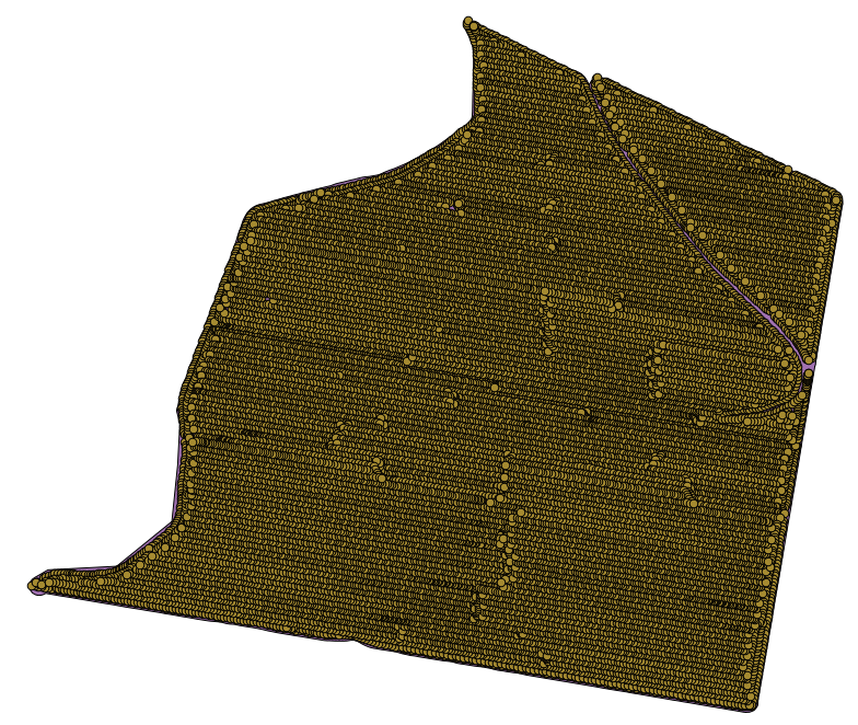
The data correspond to crop yield data, as produced by a modern harvester, and we will use it to get a raster layer of crop yield. We do not plan to do any further analysis with that layer, but just to use it as a background layer for easily identifying the most productive areas and also those where productivity can be improved.
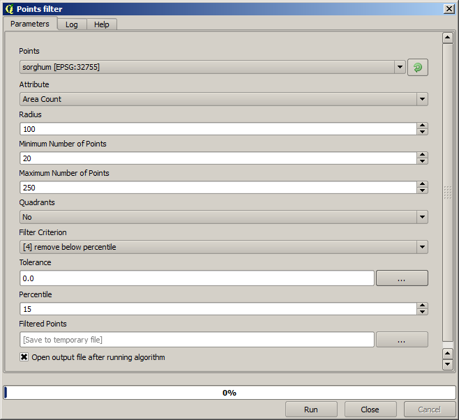
The first thing to do is to clean–up the layer, since it contains redundant points. These are caused by the movement of the harvester, in places where it has to do a turn or it changes its speed for some reason. The Points filter algorithm will be useful for this. We will use it twice, to remove points that can be considered outliers both in the upper and lower part of the distribution.
Pentru prima execuție, folosiți următoarele valori ale parametrilor.
Pentru următoarea execuție, folosiți configurația prezentată mai jos.
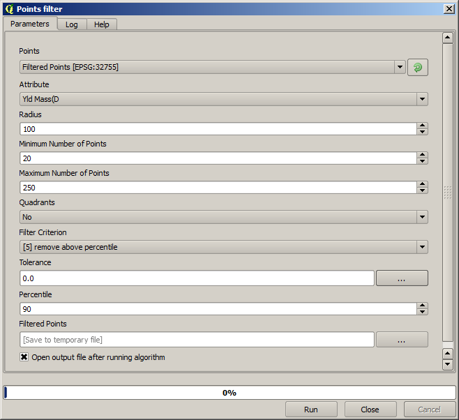
Observați că nu utilizăm stratul original ca intrare, ci rezultatul execuției anterioare în loc.
Stratul de filtrare final, cu un set redus de puncte, ar trebui să arate similar cu cel original, dar conține un număr mai mic de puncte. Puteți verifica acest lucru, prin compararea tabelelor de atribute.
Now let’s rasterize the layer using the Rasterize algorithm.
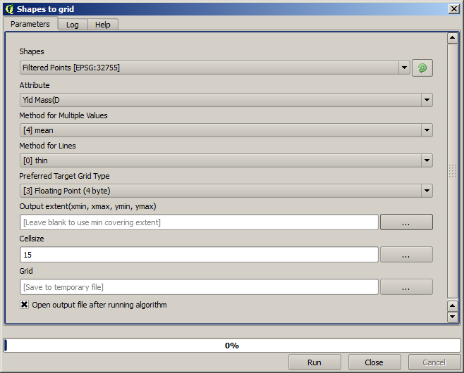
The Filtered points layer refers to the resulting one of the second filter.
It has the same name as the one produced by the first filter, since the name
is assigned by the algorithm, but you should not use the first one. Since we
will not be using it for anything else, you can safely remove it from your
project to avoid confusion, and leave just the last filtered layer.
Rezultatul raster arată în felul următor.
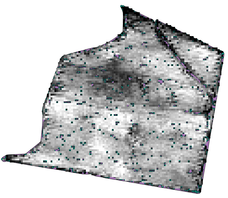
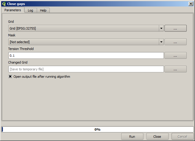
It is already a raster layer, but it is missing data in some of its cells. It only contain valid values in those cells that contained a point from the vector layer that we have just rasterized, and a no–data value in all the other ones. To fill the missing values, we can use the Close gaps algorithm.
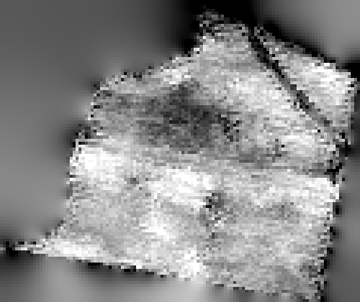
Stratul din care lipsesc valorile fără–date arată în felul următor.
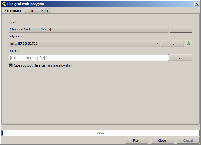
To restrict the area covered by the data to just the region where crop yield was measured, we can clip the raster layer with the provided limits layer.
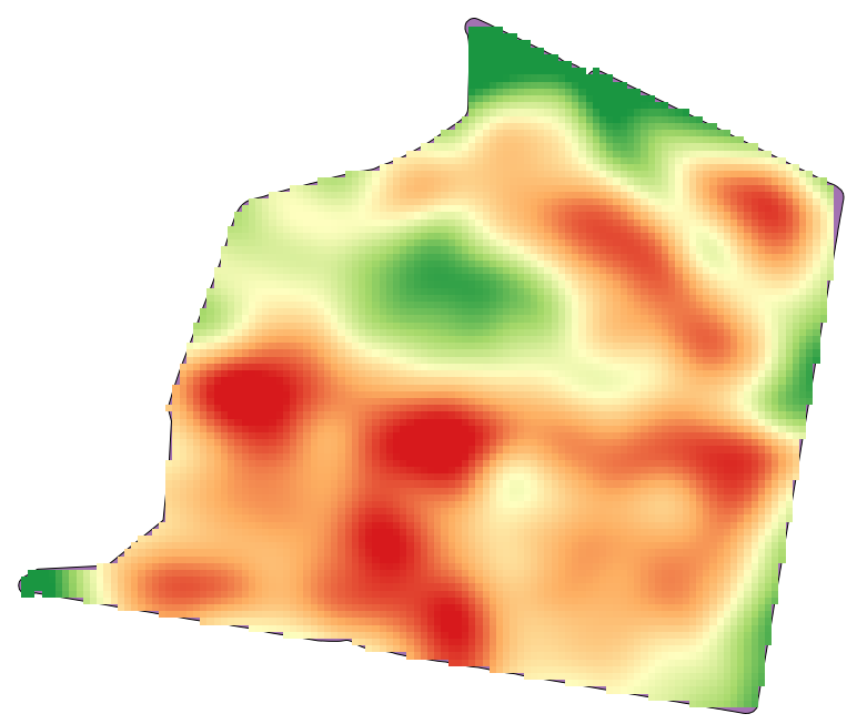
And for a smoother result (less accurate but better for rendering in the background as a support layer), we can apply a Gaussian filter to the layer.
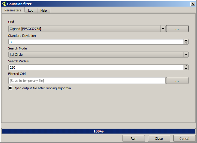
Cu parametrii de mai sus, veți primi următorul rezultat