5. Data Capture
|
Objectives: |
Learn how to create and edit vector and attribute data. |
Keywords: |
Editing, data capture, heads-up, table, database. |
5.1. Overview
In the previous two topics we looked at vector data. We saw that there are two key concepts to vector data, namely: geometry and attributes. The geometry of a vector feature describes its shape and position, while the attributes of a vector feature describe its properties (colour, size, age etc.).
In this section we will look more closely at the process of creating and editing vector data — both the geometry and attributes of vector features.
5.2. How does GIS digital data get stored?
Word processors, spreadsheets and graphics packages are all programs that let you
create and edit digital data. Each type of application saves its data into a
particular file format. For example, a graphics program will let you save your
drawing as a .jpg JPEG image, word processors let you save your document
as an .odt OpenDocument or .doc Word Document, and so on.
Just like these other applications, GIS Applications can store their data in files on the computer hard disk. There are a number of different file formats for GIS data, but the most common one is probably the ‘shape file’. The name is a little odd in that although we call it a shape file (singular), it actually consists of at least three different files that work together to store your digital vector data, as shown in Table 5.1.
Extension |
Description |
|---|---|
|
The geometry of vector features are stored in this file |
|
The attributes of vector features are stored in this file |
|
This file is an index that helps the GIS Application to find features more quickly. |
When you look at the files that make up a shapefile on the computer hard disk,
you will see something like Fig. 5.46. If you want to share vector data
stored in shapefiles with another person, it is important to give them all of
the files for that layer. So in the case of the trees layer shown in Fig. 5.46,
you would need to give the person trees.shp, trees.shx,
trees.dbf, trees.prj and trees.qml.
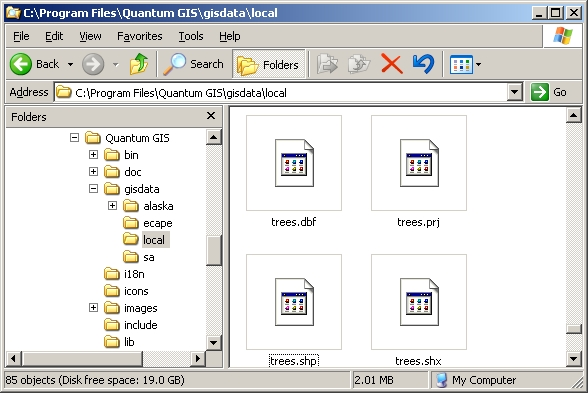
Fig. 5.46 The files that make up a ’trees’ shapefile as seen in the computer’s file manager.
Many GIS Applications are also able to store digital data inside a database. In general storing GIS data in a database is a good solution because the database can store large amounts of data efficiently and can provide data to the GIS Application quickly. Using a database also allows many people to work with the same vector data layers at the same time. Setting up a database to store GIS data is more complicated than using shapefiles, so for this topic we will focus on creating and editing shapefiles.
5.3. Planning before you begin
Before you can create a new vector layer (which will be stored in a shapefile), you need know what the geometry of that layer will be (point, polyline or polygon), and you need to know what the attributes of that layer will be. Let’s look at a few examples and it will become clearer how to go about doing this.
5.3.1. Example 1: Creating a tourism map
Imagine that you want to create a nice tourism map for your local area. Your vision of the final map is a 1:50 000 toposheet with markers overlaid for sites of interest to tourists. First, let’s think about the geometry. We know that we can represent a vector layer using point, polyline or polygon features. Which one makes the most sense for our tourism map? We could use points if we wanted to mark specific locations such as look out points, memorials, battle sites and so on. If we wanted to take tourists along a route, such as a scenic route through a mountain pass, it might make sense to use polylines. If we have whole areas that are of tourism interest, such as a nature reserve or a cultural village, polygons might make a good choice.
As you can see it’s often not easy to know what type of geometry you will need. One common approach to this problem is to make one layer for each geometry type you need. So, for example, if you look at digital data provided by the Chief Directorate: Surveys and Mapping, South Africa, they provide a river areas (polygons) layer and a rivers polyline layer. They use the river areas (polygons) to represent river stretches that are wide, and they use river polylines to represent narrow stretches of river. In Fig. 5.47 we can see how our tourism layers might look on a map if we used all three geometry types.
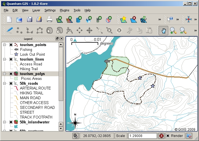
Fig. 5.47 A map with tourism layers. We have used three different geometry types for tourism data so that we can properly represent the different kinds of features needed for our visitors, giving them all the information they need.
5.3.2. Example 2: Creating a map of pollution levels along a river
If you wanted to measure pollution levels along the course of a river you would typically travel along the river in a boat or walk along its banks. At regular intervals you would stop and take various measurements such as Dissolved Oxygen (DO) levels, Coliform Bacteria (CB) counts, Turbidity levels and pH. You would also need to make a map reading of your position or obtain your position using a GPS receiver.
To store the data collected from an exercise like this in a GIS Application, you would probably create a GIS layer with a point geometry. Using point geometry makes sense here because each sample taken represents the conditions at a very specific place.
For the attributes we would want a field for each thing that describes the sample site. So we may end up with an attribute table that looks something like Table 5.2.
SampleNo |
pH |
DO |
CB |
Turbidity |
Collector |
Date |
|---|---|---|---|---|---|---|
1 |
7 |
6 |
N |
Low |
Patience |
12/01/2009 |
2 |
6.8 |
5 |
Y |
Medium |
Thabo |
12/01/2009 |
3 |
6.9 |
6 |
Y |
High |
Victor |
12/01/2009 |
Drawing a table like Table 5.2 before you create your vector layer will let you decide what attribute fields (columns) you will need. Note that the geometry (positions where samples were taken) is not shown in the attribute table — the GIS Application stores it separately!
5.4. Creating an empty shapefile
Once you have planned what features you want to capture into the GIS, and the geometry type and attributes that each feature should have, you can move on to the next step of creating an empty shapefile.
The process usually starts with choosing the ‘new vector layer’ option in your GIS Application and then selecting a geometry type (see Fig. 5.48). As we covered in an earlier topic, this means choosing either point, polyline or polygon for the geometry.
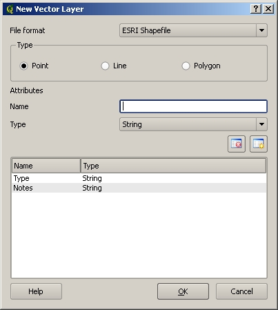
Fig. 5.48 Creating a new vector layer is as simple as filling in a few details in a form. First you choose the geometry type, and then you add the attribute fields.
Next you will add fields to the attribute table. Normally we give field names that are short, have no spaces and indicate what type of information is being stored in that field. Example field names may be ‘pH’, ‘RoofColour’, ‘RoadType’ and so on. As well as choosing a name for each field, you need to indicate how the information should be stored in that field — i.e. is it a number, a word or a sentence, or a date?
Computer programs usually call information that is made up of words or sentences ‘strings’, so if you need to store something like a street name or the name of a river, you should use ‘String’ for the field type.
The shapefile format allows you to store the numeric field information as either a whole number (integer) or a decimal number (floating point) — so you need to think before hand whether the numeric data you are going to capture will have decimal places or not.
The final step (as shown in Fig. 5.49) for creating a shapefile is to give it a name and a place on the computer hard disk where it should be created. Once again it is a good idea to give the shapefile a short and meaningful name. Good examples are ‘rivers’, ‘watersamples’ and so on.
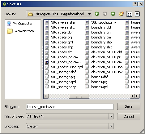
Fig. 5.49 After defining our new layer’s geometry and attributes, we need to save it to disk. It is important to give a short but meaningful name to your shapefile.
Let’s recap the process again quickly. To create a shapefile you first say what kind of geometry it will hold, then you create one or more fields for the attribute table, and then you save the shapefile to the hard disk using an easy to recognise name. Easy as 1-2-3!
5.5. Adding data to your shapefile
So far we have only created an empty shapefile. Now we need to enable editing in the shapefile using the ‘enable editing’ menu option or tool bar icon in the GIS Application. Shapefiles are not enabled for editing by default to prevent accidentally changing or deleting the data they contain. Next we need to start adding data. There are two steps we need to complete for each record we add to the shapefile:
Capturing geometry
Entering attributes
The process of capturing geometry is different for points, polylines and polygons.
To capture a point, you first use the map pan and zoom tools to get to the correct geographical area that you are going to be recording data for. Next you will need to enable the point capture tool. Having done that, the next place you click with the left mouse button in the map view, is where you want your new point geometry to appear. After you click on the map, a window will appear and you can enter all of the attribute data for that point (see Fig. 5.50). If you are unsure of the data for a given field you can usually leave it blank, but be aware that if you leave a lot of fields blank it will be hard to make a useful map from your data!
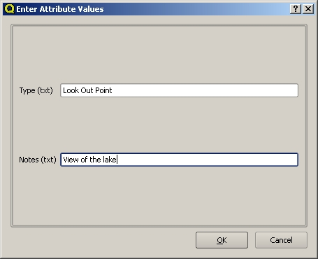
Fig. 5.50 After you have captured the point geometry, you will be asked to describe its attributes. The attribute form is based on the fields you specified when you created the vector layer.
To capture a polyline the process is similar to that of a point, in that you need to first use the pan and zoom tools to move the map in the map view to the correct geographical area. You should be zoomed in enough so that your new vector polyline feature will have an appropriate scale (see Vector Data for more details on scale issues). When you are ready, you can click the polyline capture icon in the tool bar and then start drawing your line by clicking on the map. After you make your first click, you will notice that the line stretches like an elastic band to follow the mouse cursor around as you move it. Each time you click with the left mouse button, a new vertex will be added to the map. This process is shown in Fig. 5.51.
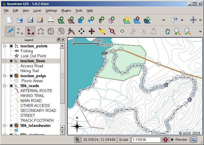
Fig. 5.51 Capturing lines for a tourism map. When editing a line layer, the vertices are shown with circular markers which you can move about with the mouse to adjust the line’s geometry. When adding a new line (shown in red), each click of the mouse will add a new vertex.
When you have finished defining your line, use the right mouse button to tell the GIS Application that you have completed your edits. As with the procedure for capturing a point feature, you will then be asked to enter in the attribute data for your new polyline feature.
The process for capturing a polygon is almost the same as capturing a polyline except that you need to use the polygon capture tool in the toolbar. Also, you will notice that when you draw your geometry on the screen, the GIS Application always creates an enclosed area.
To add a new feature after you have created your first one, you can simply click again on the map with the point, polyline or polygon capture tool active and start to draw your next feature.
When you have no more features to add, always be sure to click the ‘allow editing’ icon to toggle it off. The GIS Application will then save your newly created layer to the hard disk.
5.6. Heads-up digitising
As you have probably discovered by now if you followed the steps above, it is pretty hard to draw the features so that they are spatially correct if you do not have other features that you can use as a point of reference. One common solution to this problem is to use a raster layer (such as an aerial photograph or a satellite image) as a backdrop layer. You can then use this layer as a reference map, or even trace the features off the raster layer into your vector layer if they are visible. This process is known as ‘heads-up digitising’ and is shown in Fig. 5.52.
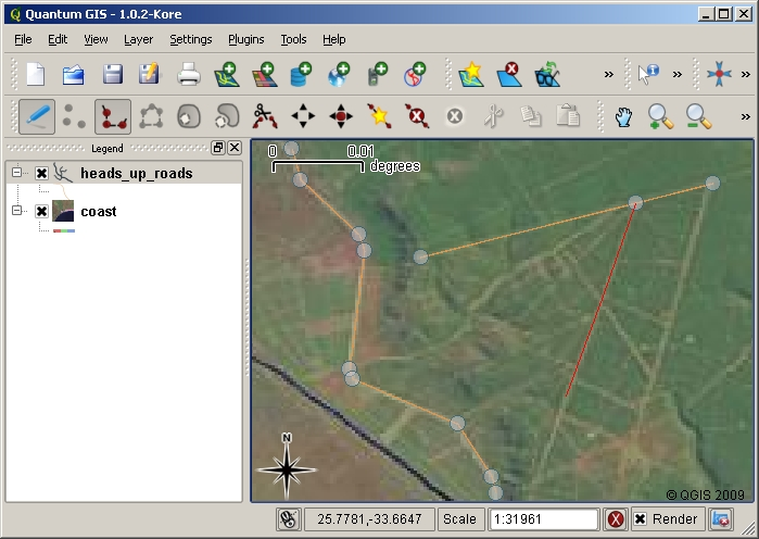
Fig. 5.52 Heads-up digitising using a satellite image as a backdrop. The image is used as a reference for capturing polyline features by tracing over them.
5.7. Digitising using a digitising table
Another method of capturing vector data is to use a digitising table. This approach is less commonly used except by GIS professionals, and it requires expensive equipment. The process of using a digitising table, is to place a paper map on the table. The paper map is held securely in place using clips. Then a special device called a ‘puck’ is used to trace features from the map. Tiny cross-hairs in the puck are used to ensure that lines and points are drawn accurately. The puck is connected to a computer and each feature that is captured using the puck gets stored in the computer’s memory. You can see what a digitising puck looks like in Fig. 5.53.

Fig. 5.53 A digitising table and puck are used by GIS professionals when they want to digitise features from existing maps.
5.8. After your features are digitised…
Once your features are digitised, you can use the techniques you learned in the previous topic to set the symbology for your layer. Choosing an appropriate symbology will allow you to better understand the data you have captured when you look at the map.
5.9. Common problems / things to be aware of
If you are digitising using a backdrop raster layer such as an aerial photograph or satellite image, it is very important that the raster layer is properly georeferenced. A layer that is georeferenced properly displays in the correct position in the map view based on the GIS Application’s internal model of the Earth. We can see the effect of a poorly georeferenced image in Fig. 5.54.
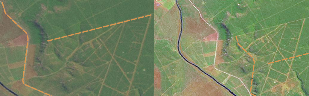
Fig. 5.54 The importance of using properly georeferenced raster images for heads-up digitising. On the left we can see the image is properly georegistered and the road features (in orange) overlap perfectly. If the image is poorly georeferenced (as shown on the right) the features will not be well aligned. Worse still, if the image on the right is used as a reference when capturing new features, the newly captured data will be inaccurate!
Also remember that it is important that you are zoomed in to an appropriate scale so that the vector features you create are useful. As we saw in the previous topic on vector geometry, it is a bad idea to digitise your data when you are zoomed out to a scale of 1:1000 000 if you intend to use the data you capture at a scale of 1:50 000 later.
5.10. What have we learned?
Let’s wrap up what we covered in this worksheet:
Digitising is the process of capturing knowledge of a feature’s geometry and attributes into a digital format stored on the computer’s disk.
GIS Data can be stored in a database or as files.
One commonly used file format is the shapefile which is actually a group of three or more files (
.shp,.dbfand.shx).Before you create a new vector layer you need to plan both what geometry type and attribute fields it will contain.
Geometry can be point, polyline or polygon.
Attributes can be integers (whole numbers), floating points (decimal numbers), strings (words) or dates.
The digitising process consists of drawing the geometry in the map view and then entering its attributes. This is repeated for each feature.
Heads-up digitising is often used to provide orientation during digitising by using a raster image in the background.
Professional GIS users sometimes use a digitising table to capture information from paper maps.
5.11. Now you try!
Here are some ideas for you to try with your learners:
Draw up a list of features in and around your school that you think would be interesting to capture. For example: the school boundary, the position of fire assembly points, the layout of each class room, and so on. Try to use a mix of different geometry types. Now split your learners into groups and assign each group a few features to capture. Have them symbolise their layers so that they are more meaningful to look at. Combine the layers from all the groups to create a nice map of your school and its surroundings!
Find a local river and take water samples along its length. Make a careful note of the position of each sample using a GPS or by marking it on a toposheet. For each sample take measurements such as pH, dissolved oxygen etc. Capture the data using the GIS application and make maps that show the samples with a suitable symbology. Could you identify any areas of concern? Was the GIS Application able to help you to identify these areas?
5.12. Something to think about
If you don’t have a computer available, you can follow the same process by using transparency sheets and a notebook. Use an aerial photo, orthosheet or satellite image printout as your background layer. Draw columns down the page in your notebook and write in the column headings for each attribute field you want to store information about. Now trace the geometry of features onto the transparency sheet, writing a number next to each feature so that it can be identified. Now write the same number in the first column in your table in your notebook, and then fill in all the additional information you want to record.
5.13. Further reading
The QGIS User Guide has more detailed information on digitising vector data in QGIS.
5.14. What’s next?
In the section that follows we will take a closer look at raster data to learn all about how image data can be used in a GIS.