Пространственный анализ векторных данных ( Буфер)¶

Обзор¶

Пространственный анализ использует пространственную составляющую данных для того, чтобы извлечь новую дополнительную информацию из них. Обычно пространтвенный анализ выполняеся ГИС программой, в которой содержатся инструменты для пространственного анализа и статистики ( например, как много вершин в полигоне) или геопроцессинга, как, например, создание буфера. Типы используемого пространнственного анализа засисят от области применения. Так, работая с управлением и исследованиями водными ресурсами (Гидрология), вероятнее всего будут испльзоватся инстументы для исследования поверхности моделирование поведения водных объектов. При управлении живой природы пользователи будут заинтересованы в аналитических функциях, которые будут описывать отношения между положением живой природы и окружающей среды. В этой теме мы будем обсуждать использование буфера как примера пространсвенного анализа векторных данных.

Создание буфера в деталях¶

Буферизация обычно создает две области: одна в пределах  указанного расстояния от выбранного объекта реального мира, другая - вне. Область, которая находится в пределах указанного расстояния называется буферная зона.

Буферная зона - область, предназначение которой отделять одни объекты реального мира от других. Часто буферные зоны используют для определения зон защиты окружающей среды, защиты жилых и коммерческих зон от промышленных аварий и природных катастроф, предотвращения насилия. Распространенным примером буферных зон будут зеленые насаджения между жилой коммерческой зонами, пограничные зоны между госудаствами ( см figure_buffer_zone), шумозащитные зоны вокруг аэропортов или зоны защиты от загрязнений вдоль рек.

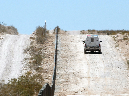
Граница между США и Мексикой разделяется буферной зоной. ( Фото сделано SGT Джим Гринхил 2006).

В приложениях ГИХ буферные зоны всегда представленны в виде векторных полигонов, которые включают в себя другие полигональные, линейные или точечные объекты ( смотрите figure_point_buffer, figure_line_buffer, ).

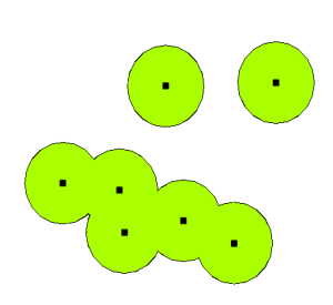
Буферная зона и векторные точки.

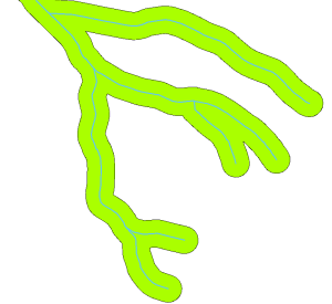
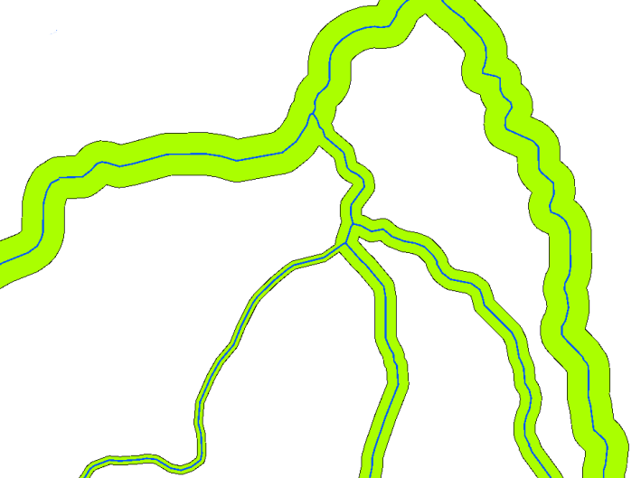
Буферная зона и векторные линии.

Буферная зона и векторные линии.

Виды буферов¶

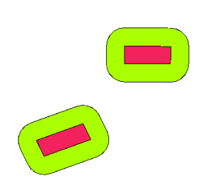
Существует несколько разновидностей буферов. Буферное расстояние или размер буфера может изменяться в зависимости от численного значения, предоставленого в таблице атрибутов векторного слоя для каждого объекта. Численные значения должны быть указаны в величинах карты в соотвестсвии с картографической проекцией, в которой хранятся данные. Например, ширина буферной зоны вдоль берегов реки может изменяться в зависимости от типа смежного землеиспользования. Для интенсивной культивации буферное расстояние может быть большим, чем для органического фермерства ( см картинку Figure figure_variable_buffer и таблицу table_buffer_attributes).

Создание буферов для реки с различным расстоянием.

Table Buffer Attributes 1: Attribute table with different buffer distances to rivers based on information about the adjacent land use.

Buffers around polyline features, such as rivers or roads, do not have to be on both sides of the lines. They can be on either the left side or the right side of the line feature. In these cases the left or right side is determined by the direction from the starting point to the end point of line during digitising.

Multiple buffer zones¶

A feature can also have more than one buffer zone. A nuclear power plant may be buffered with distances of 10, 15, 25 and 30 km, thus forming multiple rings around the plant as part of an evacuation plan (see figure_multiple_buffers).

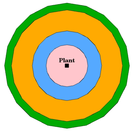
Buffering a point feature with distances of 10, 15, 25 and 30 km.

Buffering with intact or dissolved boundaries¶

Buffer zones often have dissolved boundaries so that there are no overlapping areas between the buffer zones. In some cases though, it may also be useful for boundaries of buffer zones to remain intact, so that each buffer zone is a separate polygon and you can identify the overlapping areas (see Figure figure_buffer_dissolve).

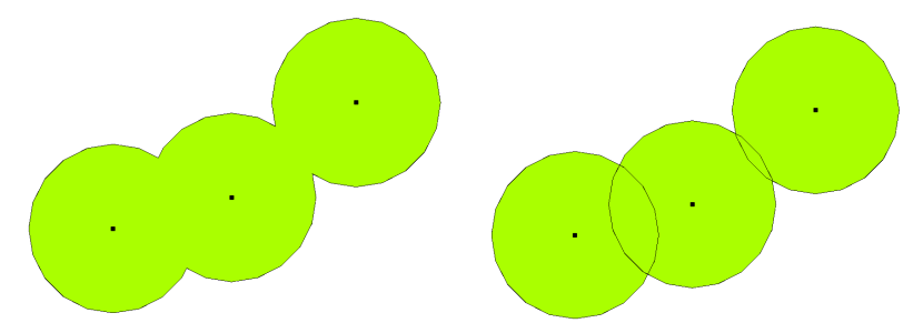
Buffer zones with dissolved (left) and with intact boundaries (right) showing overlapping areas.

Основные ошибки / о чём стоит помнить¶

Most GIS Applications offer buffer creation as an analysis tool, but the options for creating buffers can vary. For example, not all GIS Applications allow you to buffer on either the left side or the right side of a line feature, to dissolve the boundaries of buffer zones or to buffer inward from a polygon boundary.

A buffer distance always has to be defined as a whole number (integer) or a decimal number (floating point value). This value is defined in map units (meters, feet, decimal degrees) according to the Coordinate Reference System (CRS) of the vector layer.

More spatial analysis tools¶

Buffering is a an important and often used spatial analysis tool but there are many others that can be used in a GIS and explored by the user.

Spatial overlay is a process that allows you to identify the relationships between two polygon features that share all or part of the same area. The output vector layer is a combination of the input features information (see figure_overlay_operations).

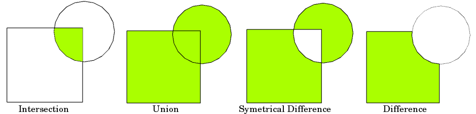
Spatial overlay with two input vector layers (a_input = rectangle, b_input = circle). The resulting vector layer is displayed green.

Typical spatial overlay examples are:

• Intersection: The output layer contains all areas where both layers overlap (intersect).
• Union: the output layer contains all areas of the two input layers combined.
• Symmetrical difference: The output layer contains all areas of the input layers except those areas where the two layers overlap (intersect).
• Difference: The output layer contains all areas of the first input layer that do not overlap (intersect) with the second input layer.

What have we learned?¶

Let’s wrap up what we covered in this worksheet:

• Buffer zones describe areas around real world features.
• Buffer zones are always vector polygons.
• A feature can have multiple buffer zones.
• The size of a buffer zone is defined by a buffer distance.
• A buffer distance has to be an integer or floating point value.
• A buffer distance can be different for each feature within a vector layer.
• Polygons can be buffered inward or outward from the polygon boundary.
• Buffer zones can be created with intact or dissolved boundaries.
• Besides buffering, a GIS usually provides a variety of vector analysis tools to solve spatial tasks.

Now you try!¶

Here are some ideas for you to try with your learners:

• Because of dramatic traffic increase, the town planners want to widen the main road and add a second lane. Create a buffer around the road to find properties that fall within the buffer zone (see figure_buffer_road).
• For controlling protesting groups, the police want to establish a neutral zone to keep protesters at least 100 meters from a building. Create a buffer around a building and colour it so that event planners can see where the buffer area is.
• A truck factory plans to expand. The siting criteria stipulate that a potential site must be within 1 km of a heavy-duty road. Create a buffer along a main road so that you can see where potential sites are.
• Imagine that the city wants to introduce a law stipulating that no bottle stores may be within a 1000 meter buffer zone of a school or a church. Create a 1 km buffer around your school and then go and see if there would be any bottle stores too close to your school.

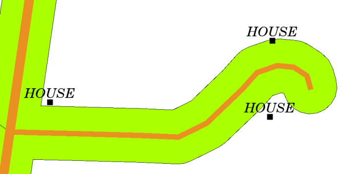
Buffer zone (green) around a roads map (brown). You can see which houses fall within the buffer zone, so now you could contact the owner and talk to him about the situation.

Something to think about¶

If you don’t have a computer available, you can use a toposheet and a compass to create buffer zones around buildings. Make small pencil marks at equal distance all along your feature using the compass, then connect the marks using a ruler!

Further reading¶

Books:

• Galati, Stephen R. (2006). Geographic Information Systems Demystified. Artech House Inc. ISBN: 158053533X
• Chang, Kang-Tsung (2006). Introduction to Geographic Information Systems. 3rd Edition. McGraw Hill. ISBN: 0070658986
• DeMers, Michael N. (2005). Fundamentals of Geographic Information Systems. 3rd Edition. Wiley. ISBN: 9814126195

Websites:

• http://www.manifold.net/doc/transform_border_buffers.htm

The QGIS User Guide also has more detailed information on analysing vector data in QGIS.

What’s next?¶

In the section that follows we will take a closer look at interpolation as an example of spatial analysis you can do with raster data.