8.3. Lesson: Analiza Terenului¶

8.3.1. Follow Along: Calculul Umbrei Versanţilor¶

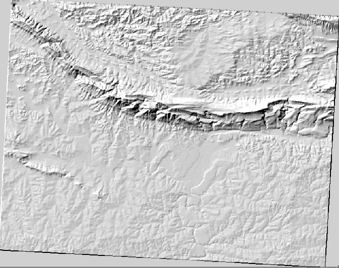
The DEM you have on your map right now does show you the elevation of the terrain, but it can sometimes seem a little abstract. It contains all the 3D information about the terrain that you need, but it doesn’t look like a 3D object. To get a better look at the terrain, it is possible to calculate a hillshade, which is a raster that maps the terrain using light and shadow to create a 3D-looking image.

To work with DEMs, you should use QGIS’ all-in-one DEM (Terrain models) analysis tool.

• Click on the menu item Raster ‣ Analysis ‣ DEM (Terrain models).
• In the dialog that appears, ensure that the Input file is the DEM layer.
• Set the Output file to hillshade.tif in the directory exercise_data/residential_development.
• Also make sure that the Mode option has Hillshade selected.
• Check the box next to Load into canvas when finished.
• You may leave all the other options unchanged.
• Click OK to generate the hillshade.
• When it tells you that processing is completed, click OK on the message to get rid of it.
• Click Close on the main DEM (Terrain models) dialog.

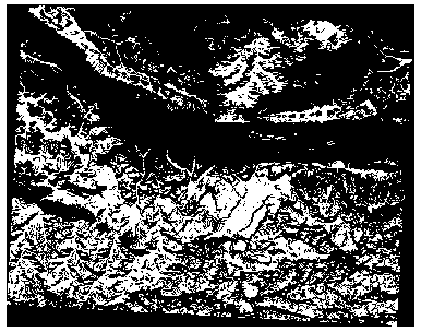
Aveți acum un nou strat denumit hillshade, care arată astfel:

That looks nice and 3D, but can we improve on this? On its own, the hillshade looks like a plaster cast. Can’t we use it together with our other, more colorful rasters somehow? Of course we can, by using the hillshade as an overlay.

8.3.2. Follow Along: Folosirea Umbrei Versanților pentru Suprapunere¶

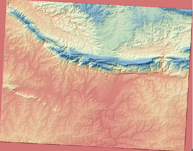
Umbra versanților poate furniza informații foarte utile despre lumina solară, la un moment dat al zilei. Ea poate fi, de asemenea, utilizată în scopuri estetice, pentru a face harta să arate mai bine. Cheia pentru acest lucru este setarea reliefului de a fi în cea mai mare parte transparent.

• Change the symbology of the original DEM to use the Pseudocolor scheme as in the previous exercise.

• Hide all the layers except the DEM and hillshade layers.

• Click and drag the DEM to be beneath the hillshade layer in the Layers list.

• Set the hillshade layer to be transparent by opening its Layer Properties and go to the Transparency tab.

• Set the Global transparency to 50%:

• Click OK on the Layer Properties dialog. You’ll get a result like this:

  

• Switch the hillshade layer off and back on in the Layers list to see the difference it makes.

Using a hillshade in this way, it’s possible to enhance the topography of the landscape. If the effect doesn’t seem strong enough to you, you can change the transparency of the hillshade layer; but of course, the brighter the hillshade becomes, the dimmer the colors behind it will be. You will need to find a balance that works for you.

Remember to save your map when you are done.

8.3.3. Follow Along: Calculul Pantei¶

În cazul unui teren, este util să-i cunoașteți panta. Dacă, de exemplu, doriți să construiți niște case pe un teren, atunci este necesar ca un teren să fie relativ plat.

To do this, you need to use the Slope mode of the DEM (Terrain models) tool.

• Open the tool as before.

• Select the Mode option Slope:

  

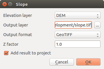
• Set the save location to exercise_data/residential_development/slope.tif

• Enable the Load into canvas... checkbox.

• Click OK and close the dialogs when processing is complete, and click Close to close the dialog. You’ll see a new raster loaded into your map.

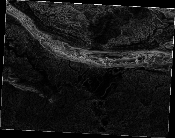
• With the new raster selected in the Layers list, click the Stretch Histogram to Full Dataset button. Now you’ll see the slope of the terrain, with black pixels being flat terrain and white pixels, steep terrain:

  

8.3.4. Try Yourself calculating the aspect¶

The aspect of terrain refers to the direction it’s facing in. Since this study is taking place in the Southern Hemisphere, properties should ideally be built on a north-facing slope so that they can remain in the sunlight.

• Use the Aspect mode of the DEM (Terain models) tool to calculate the aspect of the terrain.

Check your results

8.3.5. Follow Along: Folosirea Calculatorului Raster¶

Think back to the estate agent problem, which we last addressed in the Vector Analysis lesson. Let’s imagine that the buyers now wish to purchase a building and build a smaller cottage on the property. In the Southern Hemisphere, we know that an ideal plot for development needs to have areas on it that are north-facing, and with a slope of less than five degrees. But if the slope is less than 2 degrees, then the aspect doesn’t matter.

Fortunately, you already have rasters showing you the slope as well as the aspect, but you have no way of knowing where both conditions are satisfied at once. How could this analysis be done?

Răspunsul se află cu ajutorul: Calculatorului raster.

• Click on Raster > Raster calculator... to start this tool.
• To make use of the aspect dataset, double-click on the item aspect@1 in the Raster bands list on the left. It will appear in the Raster calculator expression text field below.

North is at 0 (zero) degrees, so for the terrain to face north, its aspect needs to be greater than 270 degrees and less than 90 degrees.

• In the Raster calculator expression field, enter this expression:

  aspect@1 <= 90 OR aspect@1 >= 270

• Set the output file to aspect_north.tif in the directory exercise_data/residential_development/.

• Ensure that the box Add result to project is checked.

• Click OK to begin processing.

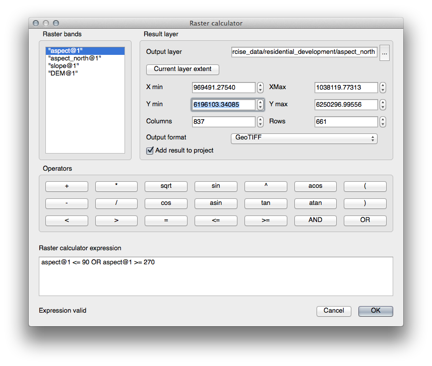
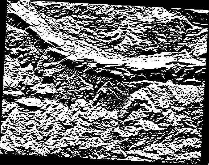
Rezultatul va fi acesta:

8.3.6. Try Yourself¶

Acum, că ați definitivat aspectul, crea două noi analize separate, ale stratului DEM.

• The first will be to identify all areas where the slope is less than or equal to 2 degrees.
• The second is similar, but the slope should be less than or equal to 5 degrees.
• Save them under exercise_data/residential_development/ as slope_lte2.tif and slope_lte5.tif.

Check your results

8.3.7. Follow Along: Combinarea Rezultatelor Analizei Raster¶

Acum aveți trei noi Analize Raster ale stratului DEM:

• aspect_north: terenul orientat spre nord

• slope_lte2: panta este la, sau sub, 2 grade

• slope_lte5: panta este la, sau sub, 5 grade

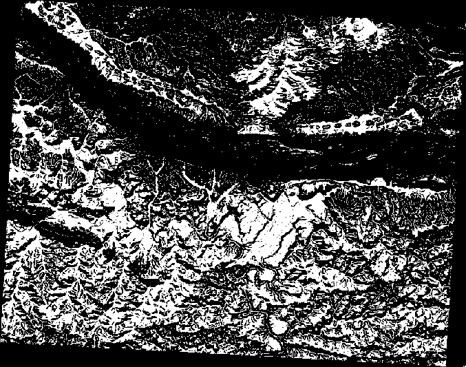
Where the conditions of these layers are met, they are equal to 1. Elsewhere, they are equal to 0. Therefore, if you multiply one of these rasters by another one, you will get the areas where both of them are equal to 1.

The conditions to be met are: at or below 5 degrees of slope, the terrain must face north; but at or below 2 degrees of slope, the direction that the terrain faces in does not matter.

Therefore, you need to find areas where the slope is at or below 5 degrees AND the terrain is facing north; OR the slope is at or below 2 degrees. Such terrain would be suitable for development.

Pentru a calcula zonele care îndeplinesc aceste criterii:

• Open your Raster calculator again.

• Use the Raster bands list, the Operators buttons, and your keyboard to build this expression in the Raster calculator expression text area:

  ( aspect_north@1 = 1 AND slope_lte5@1 = 1 )  OR slope_lte2@1 = 1

• Save the output under exercise_data/residential_development/ as all_conditions.tif.

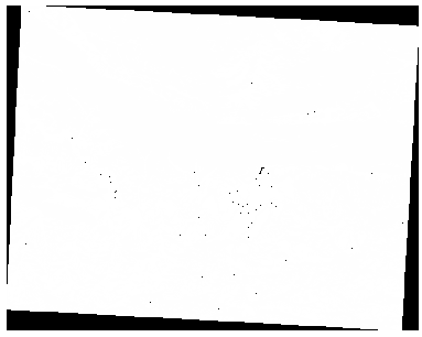
• Click OK on the Raster calculator. Your results:

  

8.3.8. Follow Along: Simplificarea Rasterului¶

As you can see from the image above, the combined analysis has left us with many, very small areas where the conditions are met. But these aren’t really useful for our analysis, since they’re too small to build anything on. Let’s get rid of all these tiny unusable areas.

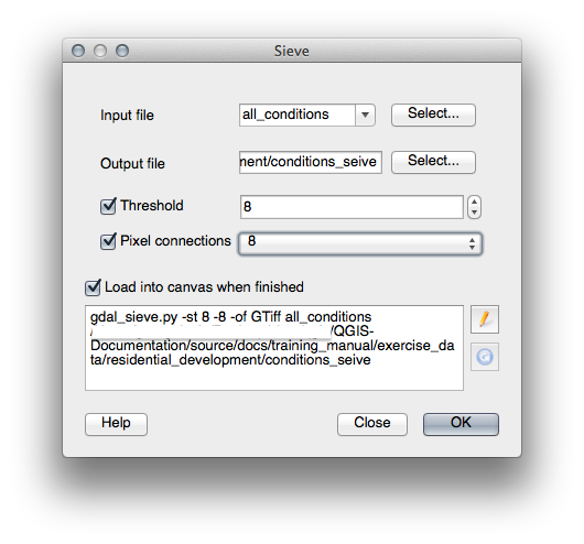
• Open the Sieve tool (Raster ‣ Analysis ‣ Sieve).
• Set the Input file to all_conditions, and the Output file to all_conditions_sieve.tif (under exercise_data/residential_development/).
• Set both the Threshold and Pixel connections values to 8, then run the tool.

Once processing is done, the new layer will load into the canvas. But when you try to use the histogram stretch tool to view the data, this happens:

Ce se întâmplă? Răspunsul se află în metadatele noului fișier raster.

• View the metadata under the Metadata tab of the Layer Properties dialog. Look in the Properties section at the bottom.

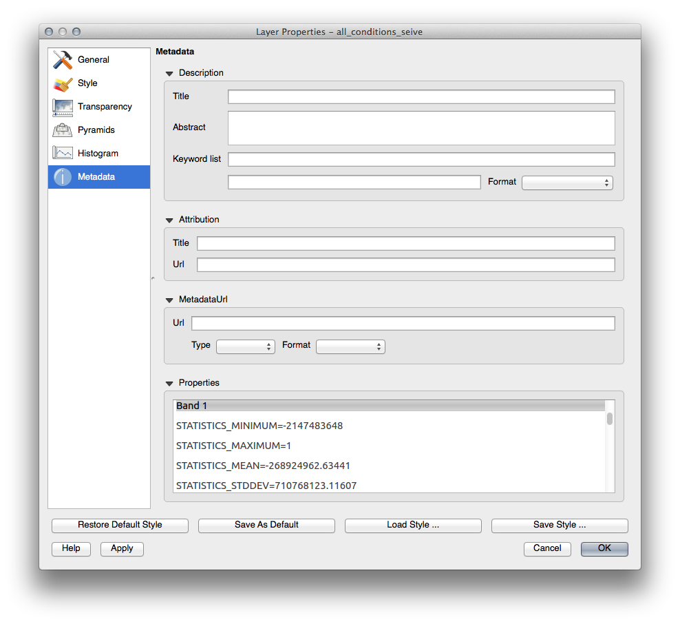
Whereas this raster, like the one it’s derived from, should only feature the values 1 and 0, it has the STATISTICS_MINIMUM value of a very large negative number. Investigation of the data shows that this number acts as a null value. Since we’re only after areas that weren’t filtered out, let’s set these null values to zero.

• Open the Raster Calculator again, and build this expression:

  (all_conditions_sieve@1 <= 0) = 0

  This will maintain all existing zero values, while also setting the negative numbers to zero; which will leave all the areas with value 1 intact.

• Save the output under exercise_data/residential_development/ as all_conditions_simple.tif.

Rezultatul dvs. arată în felul următor:

This is what was expected: a simplified version of the earlier results. Remember that if the results you get from a tool aren’t what you expected, viewing the metadata (and vector attributes, if applicable) can prove essential to solving the problem.

8.3.9. In Conclusion¶

You’ve seen how to derive all kinds of analysis products from a DEM. These include hillshade, slope and aspect calculations. You’ve also seen how to use the raster calculator to further analyze and combine these results.

8.3.10. What’s Next?¶

Now you have two analyses: the vector analysis which shows you the potentially suitable plots, and the raster analysis that shows you the potentially suitable terrain. How can these be combined to arrive at a final result for this problem? That’s the topic for the next lesson, starting in the next module.