18.17. Lucrul cu modelatorul grafic¶

O sesiune normală cu uneltele de procesare include mai mult decât rularea unui singur algoritm. De obicei, multe dintre ele sunt rulate pentru a obține o ieșire, unele dintre aceste rezultate fiind folosite ca intrare pentru alți algoritmi.

Cu ajutorul modelatorului grafic, fluxul de lucru poate fi definit într-un model, care va rula toți algoritmii necesari într-o singură execuție, simplificând și automatizând astfel întregul proces.

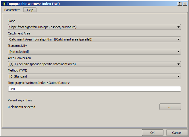
La începutul acestei lecții, vom calcula un parametru denumit Indicele Topografic de Umezeală. Algoritmul care îl calculează este denumit Indicele Topografic de Umezeală (twi)

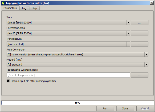
As you can see, there are two mandatory inputs: Slope and Catchment area. There is also an optional input, but we will not be using it, so we can ignore it.

The data for this lesson contains just a DEM, so we do not have any of the required inputs. However, we know how to calculate both of them from that DEM, since we have already seen the algorithms to compute slope and catchment area. So we can first compute those layers and then use them for the TWI algorithm.

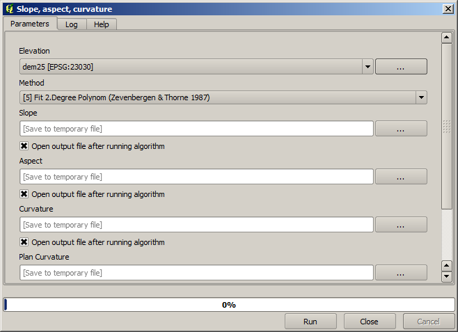
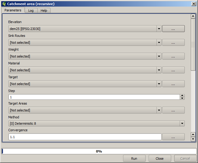
Aici sunt dialogurile pentru parametrii care ar trebui să fie utilizați în calculul a 2 straturi intermediare.

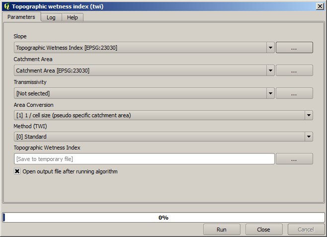
Acesta este modul în care va trebui să setați parametrii dialogului pentru algoritmul TWI.

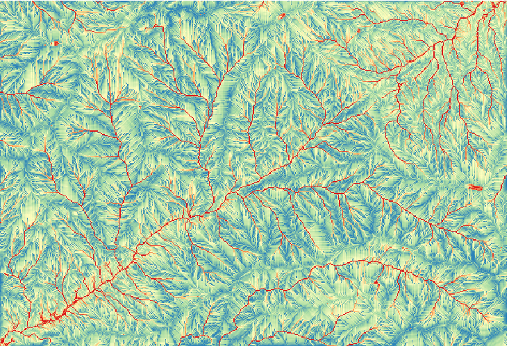
This is the result that you will obtain (the default singleband pseudocolor inverted palette has been used for rendering). You can use the twi.qml style provided.

What we will try to do now is to create an algorithm that calculates the TWI from a DEM in just one single step. That will save us work in case we later have to compute a TWI layer from another DEM, since we will need just one single step to do it instead of the 3 ones above. All the processes that we need are found in the toolbox, so what we have to do is to define the workflow to wrap them. This is where the graphical modeler comes in.

Deschideți modelatorul, prin selectarea intrării sale din meniul de prelucrare.

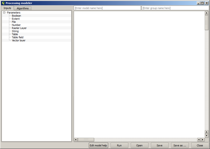
Two things are needed to create a model: setting the inputs that it will need, and defining the algorithm that it contains. Both of them are done by adding elements from the two tabs in the left–hand side of the modeler window: Inputs and Algorithms

Let’s start with the inputs. In this case we do not have much to add. We just need a raster layer with the DEM, and that will be our only input data.

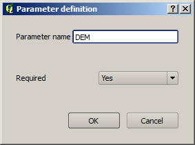
Dublu clic pe Stratul raster de intrare, apoi veți vedea următorul dialog.

Here we will have to define the input we want. Since we expect this raster layer to be a DEM, we will call it DEM. That’s the name that the user of the model will see when running it. Since we need that layer to work, we will define it as a mandatory layer.

Iată cum ar trebui să fie configurat dialogul.

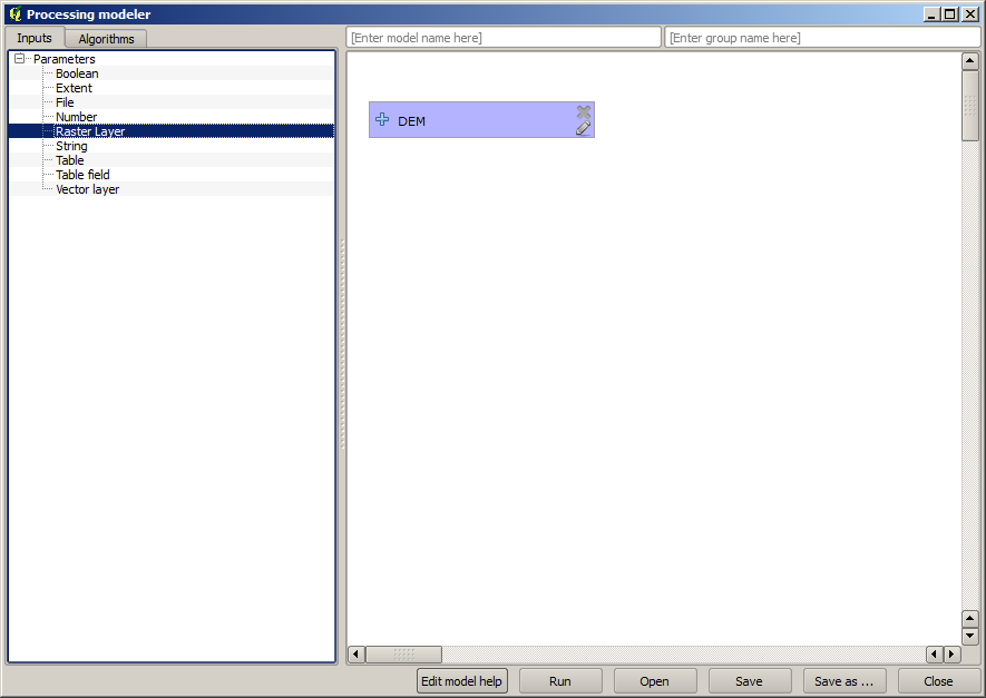
Faceți clic pe OK, după care intrarea va apărea în pânza modelatorului.

Now let’s move to the Algorithms tab. The first algorithm we have to run is the Slope, aspect, curvature algorithm. Locate it in the algorithm list, double–click on it and you will see the dialog shown below.

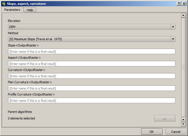
This dialog is very similar to the one that you can find when running the algorithm from the toolbox, but the element that you can use as parameter values are not taken from the current QGIS project, but from the model itself. That means that, in this case, we will not have all the raster layers of our project available for the Elevation field, but just the ones defined in our model. Since we have added just one single raster input named DEM, that will be the only raster layer that we will see in the list corresponding to the Elevation parameter.

Output generated by an algorithm are handled a bit differently when the algorithm is used as a part of a model. Instead of selecting the filepath where you want to save each output, you just have to specify if that ouput is an intermediate layer (and you do not want it to be preserved after the model has been executed), or it is a final one. In this case, all layers produced by this algorithm are intermediate. We will only use one of them (the slope layer), but we do not want to keep it, since we just need it to calculate the TWI layer, which is the final result that we want to obtain.

When layers are not a final result, you should just leave the corresponding field. Otherwise, you have to enter a name that will be used to identify the layer in the parameters dialog that will be shown when you run the model later.

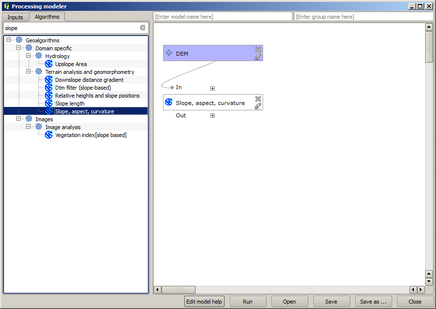
There is not much to select in this first dialog, since we do not have but just one layer in or model (The DEM input that we created). Actually, the default configuration of the dialog is the correct one in this case, so you just have to press OK. This is what you will now have in the modeler canvas.

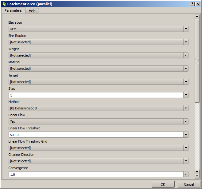
The second algorithm we have to add to our model is the catchment area algorithm. We will use the algorithm named Catchment area (Paralell). We will use the DEM layer again as input, and none of the ouputs it produces are final, so here is how you have to fill the corresponding dialog.

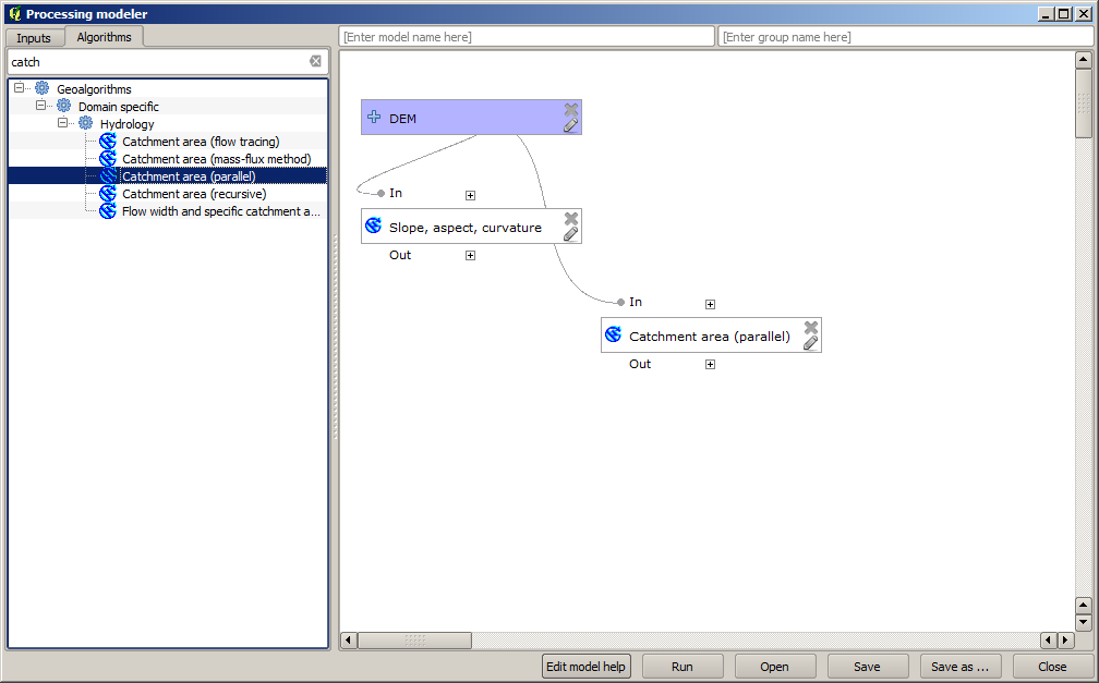
Acum, modelul dvs. ar trebui să arate în felul următor:

Ultimul pas este să adăugați algoritmul Indicelui Topografic de Umiditate, cu următoarea configurație.

In this case, we will not be using the DEM as input, but instead, we will use the slope and catchment area layers that are calculated by the algorithms that we previously added. As you add new algorithms, the outputs they produce become available for other algorithms, and using them you link the algorithms, creating the workflow.

In this case, the output TWI layer is a final layer, so we have to indicate so. In the corresponding textbox, enter the name that you want to be shown for this output.

Acum, modelul dvs. este finalizat, și ar trebui să arate în felul următor:

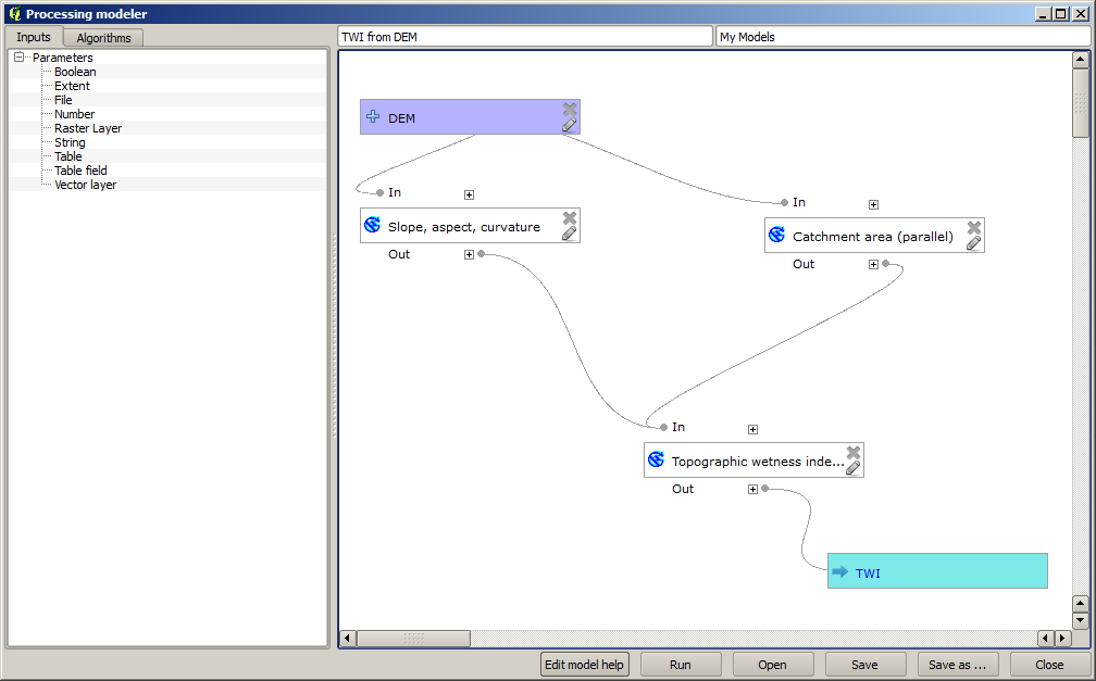
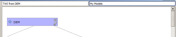
Introduceți o denumire și un nume de grup în partea de sus a ferestrei modelului, apoi salvați-l făcând clic pe butonul Save.

You can save it anywhere you want and open it later, but if you save it in the models folder (which is the folder that you will see when the save file dialog appears), you model will also be available in the toolbox as well. So stay on that folder and save the model with the filename that you prefer.

Acum închideți caseta de dialog a modelatorului și mergeți la instrumente. În Modele se va afla și modelul dvs.

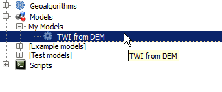
Îl puteți rula la fel ca pe oricare alt algoritm normal, printr-un dublu-clic pe el.

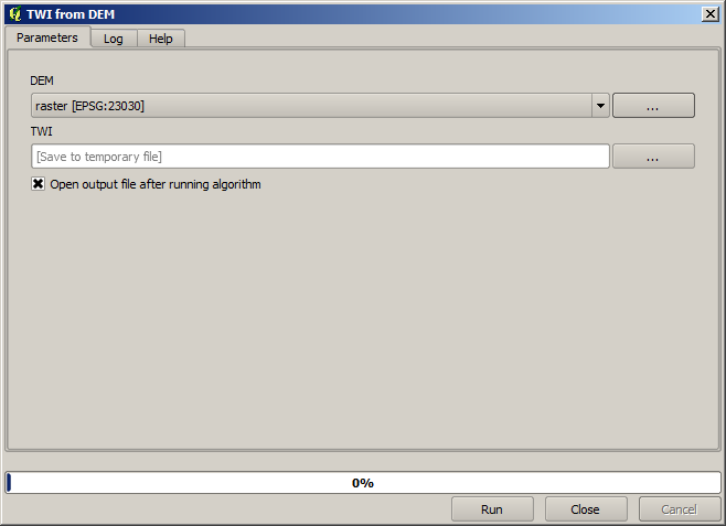
După cum puteți vedea, dialogul parametrilor, conține intrarea pe care ați adăugat-o modelului, împreună cu ieșirile pe care le stabiliți ca fiind finale, atunci când adăugați algoritmii corespunzători.

Rulați-l folosind DEM-ul ca intrare, apoi veți obține stratul TWI, într-un singur singur pas.