8.3. Lesson: Terreinanalyse
Bepaalde typen rasters stellen u in staat meer inzicht te verkrijgen over het terrein dat zij weergeven. Digital Elevation Models (DEM’s) zijn in dit opzicht in het bijzonder bruikbaar. In deze les zult u gereedschappen voor terreinanalyses gebruiken om meer uit te vinden over het te bestuderen gebied voor het eerder voorgestelde te ontwikkelen woongebied.
Het doel voor deze les: Gereedschappen voor terreinanalyses gebruiken om meer informatie over het terrein te verkrijgen.
8.3.1.  Follow Along: Een schaduw voor heuvels berekenen
The DEM you have on your map right now does show you the elevation of the terrain, but it can sometimes seem a little abstract. It contains all the 3D information about the terrain that you need, but it doesn’t look like a 3D object. To get a better look at the terrain, it is possible to calculate a hillshade, which is a raster that maps the terrain using light and shadow to create a 3D-looking image.
To work with DEMs, you should use QGIS’ all-in-one DEM (Terrain models) analysis tool.
- Click on the menu item Raster ‣ Analysis ‣ DEM (Terrain models).
- In the dialog that appears, ensure that the Input file is the DEM layer.
- Set the Output file to hillshade.tif in the directory exercise_data/residential_development.
- Also make sure that the Mode option has Hillshade selected.
- Check the box next to Load into canvas when finished.
- You may leave all the other options unchanged.
- Click OK to generate the hillshade.
- When it tells you that processing is completed, click OK on the message to get rid of it.
- Click Close on the main DEM (Terrain models) dialog.
U zult nu een nieuwe laag, genaamd hillshade, hebben die er uitziet zoals dit:
Dat ziet er leuk en 3D uit, maar kunnen we dit verbeteren? Op zichzelf ziet de schaduw voor de heuvels er uit als een gipsafdruk. Kunnen we het op een of andere manier gebruiken met onze, meer kleurrijke, rasters? Natuurlijk kunnen we dat, door de schaduw voor de heuvels er overheen te leggen.
8.3.2. Follow Along: Schaduw voor heuvels gebruiken door er overheen te leggen
Een schaduw voor heuvels kan heel bruikbare informatie verschaffen over het zonlicht op een bepaald moment van de dag. Maar het kan ook voor esthetische doeleinden gebruikt worden om de kaart er beter uit te laten zien. De sleutel hiertoe is de schaduw voor de heuvels in te stellen op bijna geheel transparant.
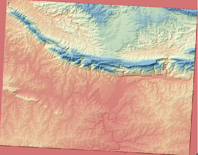
Change the symbology of the original DEM to use the Pseudocolor scheme as in the previous exercise.
Hide all the layers except the DEM and hillshade layers.
Click and drag the DEM to be beneath the hillshade layer in the Layers list.
Set the hillshade layer to be transparent by opening its Layer Properties and go to the Transparency tab.
Set the Global transparency to 50%:
Click OK on the Layer Properties dialog. You’ll get a result like this:
Switch the hillshade layer off and back on in the Layers list to see the difference it makes.
Met het op deze manier gebruiken van een schaduw voor heuvels, is het mogelijk de topografie van het landschap te verbeteren. Als het effect voor u niet sterk genoeg lijkt te zijn, kunt u de transparantie van de laag hillshade vergroten; maar natuurlijk geldt: hoe helderder de schaduw van de heuvels wordt, hoe vager de kleuren erachter zullen zijn. U dient een balans te vinden die voor u werkt.
Remember to save your map when you are done.
Notitie
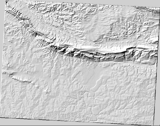
For the next two exercises, please use a new map. Load only the DEM raster dataset into it (exercise_data/raster/SRTM/srtm_41_19.tif). This is to simplify matters while you’re working with the raster analysis tools. Save the map as exercise_data/raster_analysis.qgs.
8.3.3.  Follow Along: Berekenen van de helling
Een ander handig ding om te weten van het terrein is hoe steil het is. Als u bijvoorbeeld huizen wilt bouwen op het land daar, heeft u land nodig dat relatief vlak is.
To do this, you need to use the Slope mode of the DEM (Terrain models) tool.
Open the tool as before.
Select the Mode option Slope:
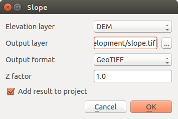
Set the save location to exercise_data/residential_development/slope.tif
Enable the Load into canvas... checkbox.
Click OK and close the dialogs when processing is complete, and click Close to close the dialog. You’ll see a new raster loaded into your map.
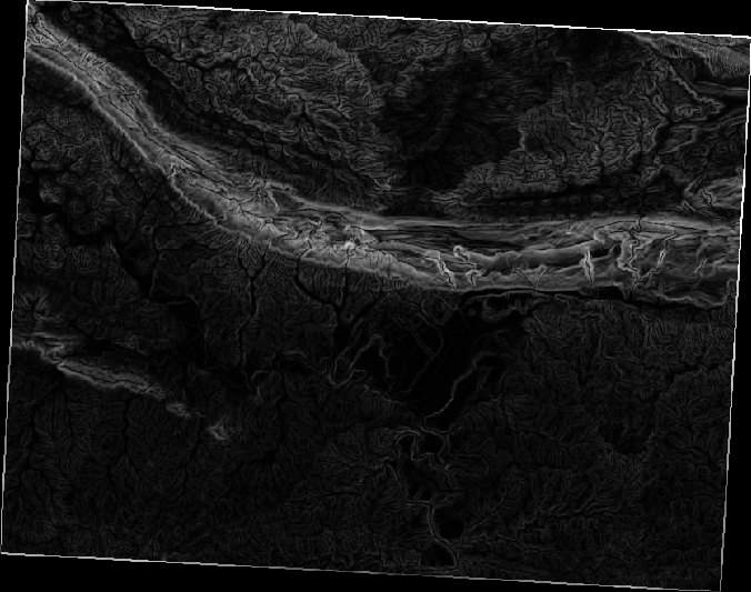
With the new raster selected in the Layers list, click the Stretch Histogram to Full Dataset button. Now you’ll see the slope of the terrain, with black pixels being flat terrain and white pixels, steep terrain:
8.3.4. Try Yourself calculating the aspect
The aspect of terrain refers to the direction it’s facing in. Since this study is taking place in the Southern Hemisphere, properties should ideally be built on a north-facing slope so that they can remain in the sunlight.
- Use the Aspect mode of the DEM (Terain models) tool to calculate the aspect of the terrain.
8.3.5. Follow Along: Rasterberekeningen gebruiken
Denk even terug aan het probleem van de makelaar dat we bespraken in de les Vectoranalyse. Laten we ons eens voorstellen dat de kopers een gebouw willen kopen en een kleinere woning willen bouwen op het land. We weten dat, in de zuidelijke hemisfeer, een ideaal gebied voor ontwikkeling gebieden moet hebben die uitkijken op het noorden, en met een helling van minder dan vijf graden. Maar als de helling minder is dan 2 graden, dan is het aspect niet van belang.
Gelukkig heeft u al rasters die u zowel de helling als het aspect weergeven, maar u heeft geen manier om te weten te komen waar aan beide voorwaarden tegelijkertijd wordt voldaan. Hoe zou deze analyse worden uitgevoerd?
Het antwoord ligt in de Rasterberekeningen.
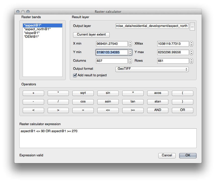
- Click on Raster > Raster calculator... to start this tool.
- To make use of the aspect dataset, double-click on the item aspect@1 in the Raster bands list on the left. It will appear in the Raster calculator expression text field below.
North is at 0 (zero) degrees, so for the terrain to face north, its aspect needs to be greater than 270 degrees and less than 90 degrees.
In the Raster calculator expression field, enter this expression:
aspect@1 <= 90 OR aspect@1 >= 270
Set the output file to aspect_north.tif in the directory exercise_data/residential_development/.
Ensure that the box Add result to project is checked.
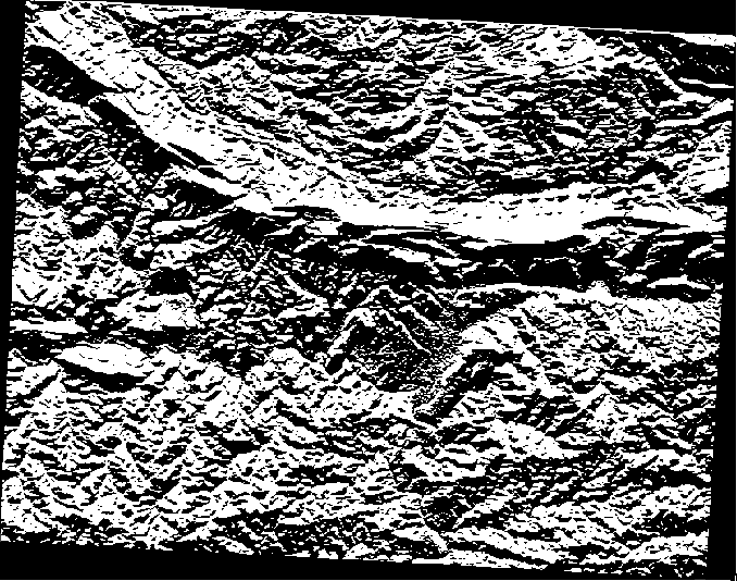
Click OK to begin processing.
Uw resultaat zal dit zijn:
8.3.6. Try Yourself
Nu u het aspect heeft gedaan, maak twee afzonderlijke nieuwe analyses van de laag DEM.
- The first will be to identify all areas where the slope is less than or equal to 2 degrees.
- The second is similar, but the slope should be less than or equal to 5 degrees.
- Save them under exercise_data/residential_development/ as slope_lte2.tif and slope_lte5.tif.
8.3.7. Follow Along: Resultaten van rasteranalyses combineren
U heeft nu drie nieuwe analyse-rasters van de laag DEM:
aspect_north: het terrein kijkt uit op het noorden
slope_lte2: de helling is 2 graden of minder
slope_lte5: de helling is 5 graden of minder
Where the conditions of these layers are met, they are equal to 1. Elsewhere, they are equal to 0. Therefore, if you multiply one of these rasters by another one, you will get the areas where both of them are equal to 1.
De voorwaarden waaraan voldaan moet worden zijn: 5 graden helling of minder, het terrein moet uitkijken op het noorden; maar bij 2 graden of minder helling is de richting waarop het terrein uitkijkt niet van belang.
Therefore, you need to find areas where the slope is at or below 5 degrees AND the terrain is facing north; OR the slope is at or below 2 degrees. Such terrain would be suitable for development.
De gebieden berekenen die voldoen aan deze criteria:
Open your Raster calculator again.
Use the Raster bands list, the Operators buttons, and your keyboard to build this expression in the Raster calculator expression text area:
( aspect_north@1 = 1 AND slope_lte5@1 = 1 ) OR slope_lte2@1 = 1
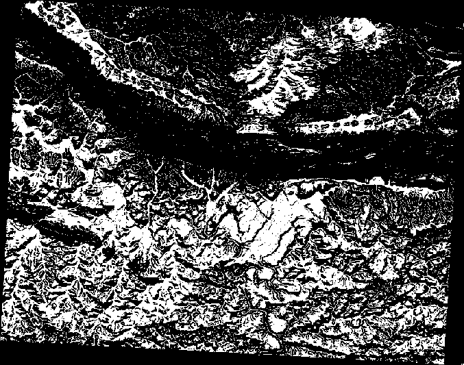
Save the output under exercise_data/residential_development/ as all_conditions.tif.
Click OK on the Raster calculator. Your results:
8.3.8. Follow Along: Het rastervereenvoudigen
Zoals u in bovenstaande afbeelding kunt zien, staan in de gecombineerde analyse vele, kleine gebieden die voldoen aan de voorwaarden. Maar deze zijn niet echt bruikbaar voor onze analyse, omdat ze te klein zijn om er iets op te bouwen. Laten we deze kleine onbruikbare gebieden verwijderen.
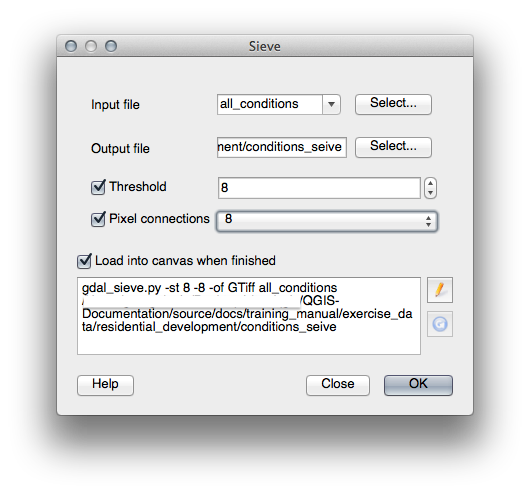
- Open the Sieve tool (Raster ‣ Analysis ‣ Sieve).
- Set the Input file to all_conditions, and the Output file to all_conditions_sieve.tif (under exercise_data/residential_development/).
- Set both the Threshold and Pixel connections values to 8, then run the tool.
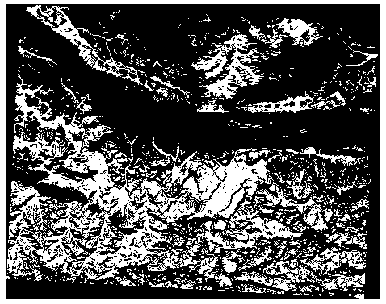
Once processing is done, the new layer will load into the canvas. But when you try to use the histogram stretch tool to view the data, this happens:

Wat is er aan de hand? Het antwoord ligt in de metadata van het nieuwe rasterbestand.
- View the metadata under the Metadata tab of the Layer Properties dialog. Look in the Properties section at the bottom.
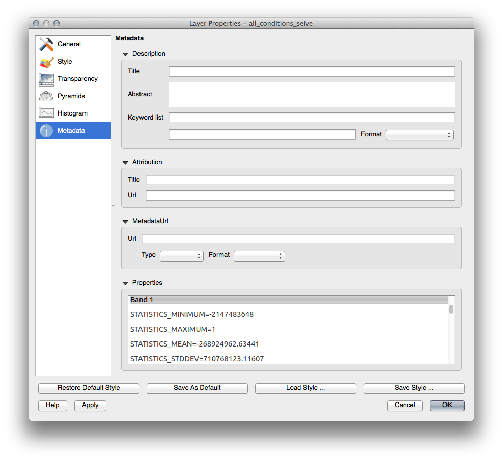
Whereas this raster, like the one it’s derived from, should only feature the values 1 and 0, it has the STATISTICS_MINIMUM value of a very large negative number. Investigation of the data shows that this number acts as a null value. Since we’re only after areas that weren’t filtered out, let’s set these null values to zero.
Open the Raster Calculator again, and build this expression:
(all_conditions_sieve@1 <= 0) = 0
This will maintain all existing zero values, while also setting the negative numbers to zero; which will leave all the areas with value 1 intact.
Save the output under exercise_data/residential_development/ as all_conditions_simple.tif.
Uw uitvoer ziet er uit zoals dit:
Dit is wat er verwacht werd: een vereenvoudigde versie van de eerdere resultaten. Onthoud dat als de resultaten die u van een gereedschap krijgt niet zijn wat u er van verwacht, het bekijken van de metadata (en vectorattributen indien van toepassing) essentieel kan blijken te zijn om het probleem op te lossen.
8.3.9. In Conclusion
You’ve seen how to derive all kinds of analysis products from a DEM. These include hillshade, slope and aspect calculations. You’ve also seen how to use the raster calculator to further analyze and combine these results.
8.3.10. What’s Next?
Nu heeft u twee analyses: de vectoranalyse die u de potentieel geschikte bouwplaatsen laat zien, en de rasteranalyse die u het potentieel geschikte terrein laat zien. Hoe kunnen deze worden gecombineerd om tot een uiteindelijk resultaat voor dit rp0obleem te komen? Dat is het onderwerp voor de volgende les, die begint in de volgende module.