8.3. Lesson: Análisis del Terreno
Ciertos tipos de ráster te permiten obtener una visión más clara del terreno que representan. Los Modelos de Digital de Elevaciones (MDEs) son particularmente útiles para ello. En esta lección utilizaras herramientas de análisis de terrenos para obtener más información sobre el área de estudio para la propuesta de desarrollo residencial anterior.
El objetivo de esta lección: Utilizar herramientas de análisis del terreno para obtener más información sobre el terreno.
8.3.1.  Follow Along: Cálculo del Relieve Sombreado
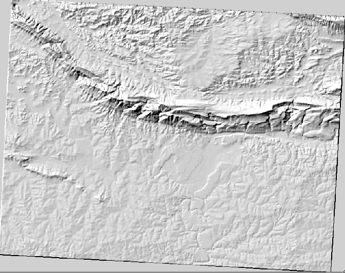
The DEM you have on your map right now does show you the elevation of the terrain, but it can sometimes seem a little abstract. It contains all the 3D information about the terrain that you need, but it doesn’t look like a 3D object. To get a better look at the terrain, it is possible to calculate a hillshade, which is a raster that maps the terrain using light and shadow to create a 3D-looking image.
To work with DEMs, you should use QGIS’ all-in-one DEM (Terrain models) analysis tool.
- Click on the menu item Raster ‣ Analysis ‣ DEM (Terrain models).
- In the dialog that appears, ensure that the Input file is the DEM layer.
- Set the Output file to hillshade.tif in the directory exercise_data/residential_development.
- Also make sure that the Mode option has Hillshade selected.
- Check the box next to Load into canvas when finished.
- You may leave all the other options unchanged.
- Click OK to generate the hillshade.
- When it tells you that processing is completed, click OK on the message to get rid of it.
- Click Close on the main DEM (Terrain models) dialog.
Ahora tendrás una capa nueva llamada relieve_sombreado que tiene este aspecto:
Se ve bien en 3D, pero ¿podemos mejorarla? En sí mismo, el sombreado del relieve parece un molde de yeso. ¿No podríamos utilizarlo con nuestros otros ráster más coloridos de alguna manera? Por supuesto que podemos, utilizando el sombreado del relieve como una capa sobrepuesta.
8.3.2. Follow Along: Utilizando un Sombreado del Relieve como Capa Sobrepuesta
Un sombreado del relieve puede proporcionar información muy útil sobre la luz solar en un momento dado del día. Pero también puede ser utilizado para fines estéticos, para que el mapa tenga mejor aspecto. La clave en este caso está en que el sombreado del relieve sea defina como mayormente transparente.
Change the symbology of the original DEM to use the Pseudocolor scheme as in the previous exercise.
Hide all the layers except the DEM and hillshade layers.
Click and drag the DEM to be beneath the hillshade layer in the Layers list.
Set the hillshade layer to be transparent by opening its Layer Properties and go to the Transparency tab.
Set the Global transparency to 50%:
Click OK on the Layer Properties dialog. You’ll get a result like this:
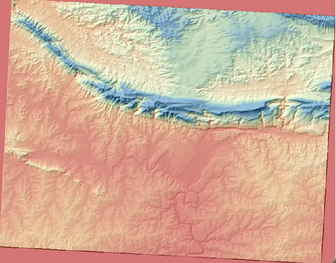
Switch the hillshade layer off and back on in the Layers list to see the difference it makes.
Utilizando el sombreado del relieve de esta forma, es posible enaltecer la topografía del paisaje. Si el efecto no parece ser suficiente para ti, puedes cambiar la transparencia de la capa relieve_sombreado, pero por supuesto, cuanto más brillante se vuelva el sombreado del relieve, peor se verán los colores bajo él. Necesitarás encontrar un balance que funcione.
Remember to save your map when you are done.
Nota
For the next two exercises, please use a new map. Load only the DEM raster dataset into it (exercise_data/raster/SRTM/srtm_41_19.tif). This is to simplify matters while you’re working with the raster analysis tools. Save the map as exercise_data/raster_analysis.qgs.
8.3.3.  Follow Along: Calculo de la Pendiente
Otra cosa útil a saber sobre el terreno es cómo de escarpado es. Si, por ejemplo, quieres construir casas en esas tierras, entonces necesitarás un terreno relativamente plano.
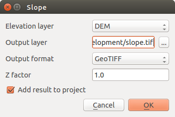
To do this, you need to use the Slope mode of the DEM (Terrain models) tool.
Open the tool as before.
Select the Mode option Slope:
Set the save location to exercise_data/residential_development/slope.tif
Enable the Load into canvas... checkbox.
Click OK and close the dialogs when processing is complete, and click Close to close the dialog. You’ll see a new raster loaded into your map.
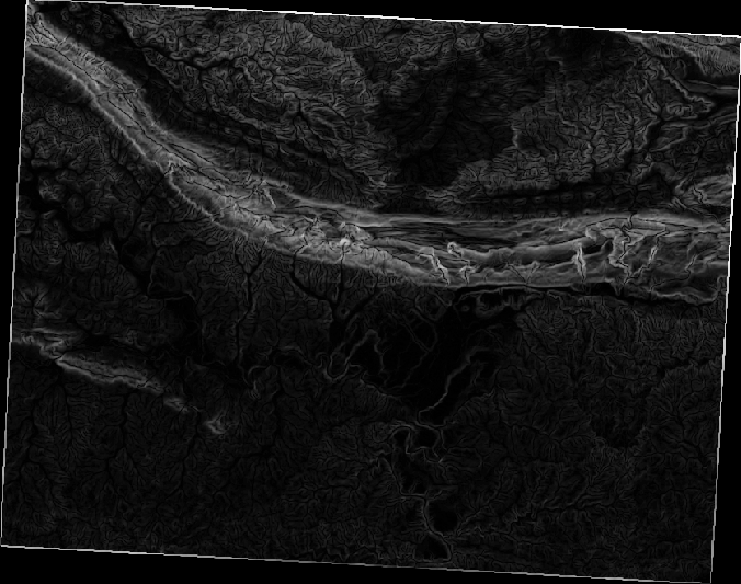
With the new raster selected in the Layers list, click the Stretch Histogram to Full Dataset button. Now you’ll see the slope of the terrain, with black pixels being flat terrain and white pixels, steep terrain:
8.3.4. Try Yourself calculating the aspect
The aspect of terrain refers to the direction it’s facing in. Since this study is taking place in the Southern Hemisphere, properties should ideally be built on a north-facing slope so that they can remain in the sunlight.
- Use the Aspect mode of the DEM (Terain models) tool to calculate the aspect of the terrain.
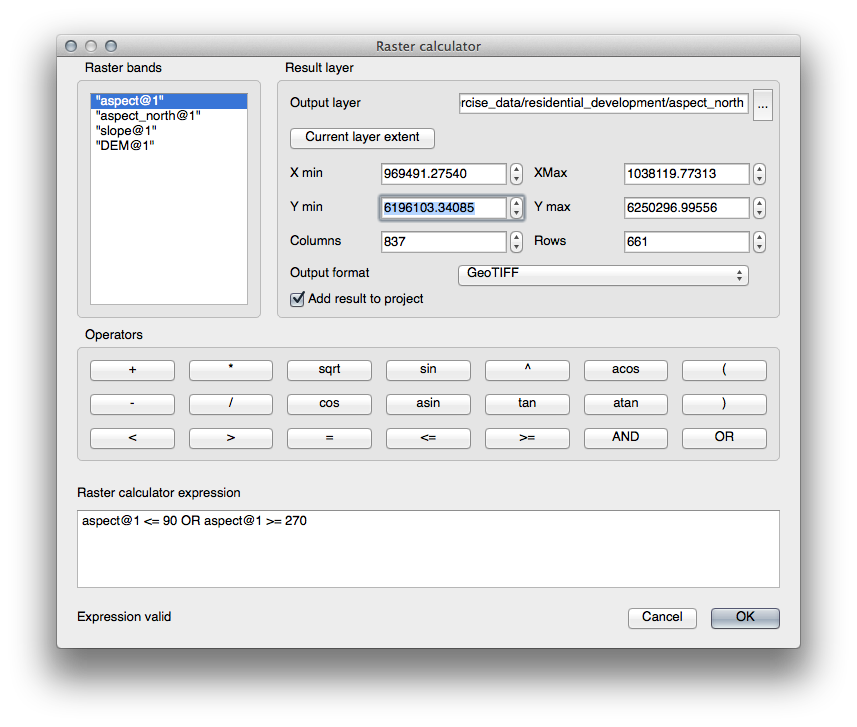
8.3.5. Follow Along: Utilizando la Calculadora Ráster
Piensa en el problema del agente inmobiliario anterior, que se abordó en la lección Análisis Vectorial. Imagina que los compradores ahora quieren encontrar una construcción y construir una pequeña casa de campo en la propiedad. En el Hemisferio Sur, sabemos que una parcela con un desarrollo ideal debe estar orientada al norte, y con una pendiente de menos de cinco grados. Pero si la pendiente es menor a 2 grados, la orientación no importará.
Afortunadamente, ya tienes rásters mostrándote la pendiente además de la orientación, pero no tienes ninguna forma de saber dónde se dan ambas condiciones a la vez. ¿Cómo se podría realizar este análisis?
La respuesta está en la Calculadora ráster.
- Click on Raster > Raster calculator... to start this tool.
- To make use of the aspect dataset, double-click on the item aspect@1 in the Raster bands list on the left. It will appear in the Raster calculator expression text field below.
North is at 0 (zero) degrees, so for the terrain to face north, its aspect needs to be greater than 270 degrees and less than 90 degrees.
In the Raster calculator expression field, enter this expression:
aspect@1 <= 90 OR aspect@1 >= 270
Set the output file to aspect_north.tif in the directory exercise_data/residential_development/.
Ensure that the box Add result to project is checked.
Click OK to begin processing.
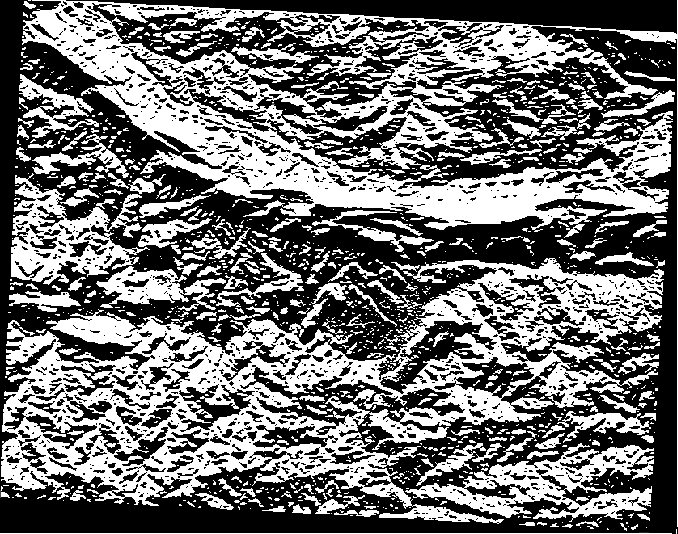
Tu resultado será este:
8.3.6. Try Yourself
Ahora que has hecho la orientación, crea dos nuevos análisis de la capa MDE.
- The first will be to identify all areas where the slope is less than or equal to 2 degrees.
- The second is similar, but the slope should be less than or equal to 5 degrees.
- Save them under exercise_data/residential_development/ as slope_lte2.tif and slope_lte5.tif.
8.3.7. Follow Along: Combinando Resultados de Análisis Ráster
Ahora tienes tres nuevos análisis ráster de la capa MDE
orientacion_norte: el terreno orientado al norte
pendiente_lte2: la pendiente igual o menor a 2 grados
pendiente_lte5: la pendiente igual o menor a 5 grados
Where the conditions of these layers are met, they are equal to 1. Elsewhere, they are equal to 0. Therefore, if you multiply one of these rasters by another one, you will get the areas where both of them are equal to 1.
Las condiciones a cumplir son; a pendientes iguales o menores de 5 grados, el terreno debe estar orientado al norte; pero a pendientes iguales o menores de 2 grados, la dirección a la que se orienta el terreno no importa.
Therefore, you need to find areas where the slope is at or below 5 degrees AND the terrain is facing north; OR the slope is at or below 2 degrees. Such terrain would be suitable for development.
Para calcular las áreas que cumplen esos criterios:
Open your Raster calculator again.
Use the Raster bands list, the Operators buttons, and your keyboard to build this expression in the Raster calculator expression text area:
( aspect_north@1 = 1 AND slope_lte5@1 = 1 ) OR slope_lte2@1 = 1
Save the output under exercise_data/residential_development/ as all_conditions.tif.
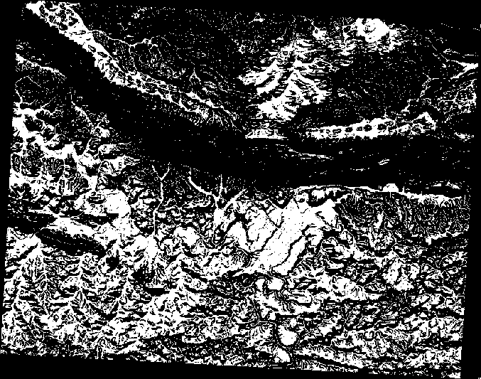
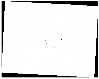
Click OK on the Raster calculator. Your results:
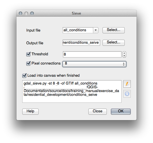
8.3.8. Follow Along: Simplificando el Ráster
Como puedes ver en la imagen superior, los análisis combinados nos dejan con muchas áreas pequeñas donde se cumplen las condiciones. Pero esas no son realmente útiles para nuestro análisis, ya que son demasiado pequeñas para construir. Vamos a deshacernos de todas esas áreas minúsculas.
- Open the Sieve tool (Raster ‣ Analysis ‣ Sieve).
- Set the Input file to all_conditions, and the Output file to all_conditions_sieve.tif (under exercise_data/residential_development/).
- Set both the Threshold and Pixel connections values to 8, then run the tool.
Once processing is done, the new layer will load into the canvas. But when you try to use the histogram stretch tool to view the data, this happens:
¿Qué está pasando? La respuesta se encuentra en los metadatos del nuevo archivo ráster.
- View the metadata under the Metadata tab of the Layer Properties dialog. Look in the Properties section at the bottom.
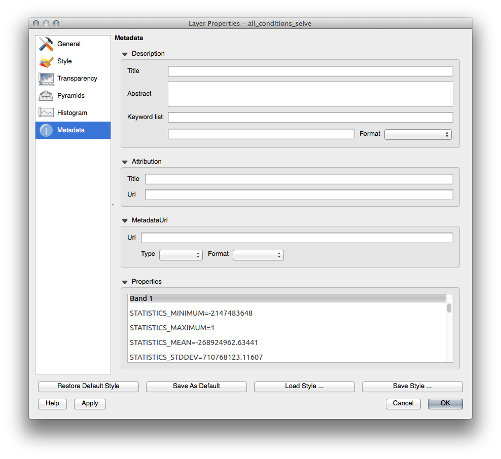
Whereas this raster, like the one it’s derived from, should only feature the values 1 and 0, it has the STATISTICS_MINIMUM value of a very large negative number. Investigation of the data shows that this number acts as a null value. Since we’re only after areas that weren’t filtered out, let’s set these null values to zero.
Open the Raster Calculator again, and build this expression:
(all_conditions_sieve@1 <= 0) = 0
This will maintain all existing zero values, while also setting the negative numbers to zero; which will leave all the areas with value 1 intact.
Save the output under exercise_data/residential_development/ as all_conditions_simple.tif.
Tu resultado tiene este aspecto:
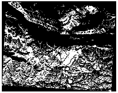
Eso era lo que se esperaba: una versión simplificada de los resultados anteriores. Recuerda que si los resultados que obtienes de una herramienta no son los que esperabas, comprobando los metadatos (y atributos vectoriales, si es aplicable) puede ser esencial para solucionar el problema.
8.3.9. In Conclusion
You’ve seen how to derive all kinds of analysis products from a DEM. These include hillshade, slope and aspect calculations. You’ve also seen how to use the raster calculator to further analyze and combine these results.
8.3.10. What’s Next?
Ahora tienes dos análisis: el análisis vectorial que te muestra las parcelas potencialmente adecuadas, y el análisis ráster que te muestra el terreno potencialmente adecuado. ¿Cómo se pueden combinar para llegar a un resultado final para este problema? Ese es el tema de la siguiente lección, empezando en el módulo siguiente.