8.3. Lesson: Analyse de terrain¶

8.3.1. Follow Along: Calcul d’un Ombrage¶

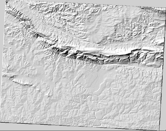
The DEM you have on your map right now does show you the elevation of the terrain, but it can sometimes seem a little abstract. It contains all the 3D information about the terrain that you need, but it doesn’t look like a 3D object. To get a better look at the terrain, it is possible to calculate a hillshade, which is a raster that maps the terrain using light and shadow to create a 3D-looking image.

To work with DEMs, you should use QGIS’ all-in-one DEM (Terrain models) analysis tool.

• Click on the menu item Raster ‣ Analysis ‣ DEM (Terrain models).
• In the dialog that appears, ensure that the Input file is the DEM layer.
• Set the Output file to hillshade.tif in the directory exercise_data/residential_development.
• Also make sure that the Mode option has Hillshade selected.
• Check the box next to Load into canvas when finished.
• You may leave all the other options unchanged.
• Click OK to generate the hillshade.
• When it tells you that processing is completed, click OK on the message to get rid of it.
• Click Close on the main DEM (Terrain models) dialog.

Vous aurez maintenant une nouvelle couche appelée hillshade qui ressemble à cela :

Le résultat semble sympathique et en 3D. Mais pouvons-nous l’améliorer ? L’ombrage semble un peut en plâtre. Pouvons-nous le combiner avec nos autres rasters plus colorés ? C’est effectivement possible en utilisant l’ombrage en tant que couverture.

8.3.2. Follow Along: Utilisation d’un ombrage comme une couverture¶

Un ombrage peut fournir des informations très utiles sur la lumière du soleil à un moment donné de la journée. Mais il peut aussi être utilisé à des fins esthétiques, pour donner à la carte une meilleure apparence. La clé pour cela est de configurer l’ombrage pour qu’il soit presque complètement transparent.

• Change the symbology of the original DEM to use the Pseudocolor scheme as in the previous exercise.

• Hide all the layers except the DEM and hillshade layers.

• Click and drag the DEM to be beneath the hillshade layer in the Layers list.

• Set the hillshade layer to be transparent by opening its Layer Properties and go to the Transparency tab.

• Set the Global transparency to 50%:

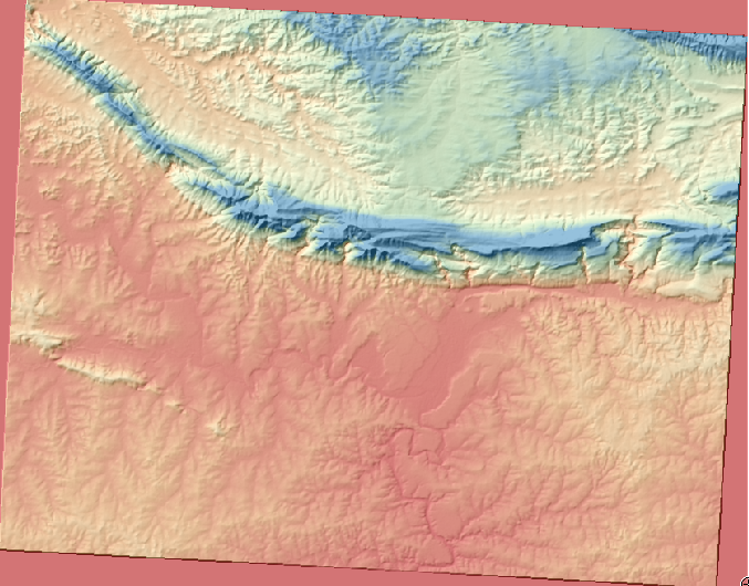
• Click OK on the Layer Properties dialog. You’ll get a result like this:

  

• Switch the hillshade layer off and back on in the Layers list to see the difference it makes.

En utilisant un ombrage de cette façon, il est possible d’améliorer la topographie du paysage. Si l’effet ne vous semble pas suffisamment fort, vous pouvez changer la transparence de la couche hillshade ; mais bien sûr que plus l’ombrage devient brillant, plus les couleurs derrière lui seront sombres. Vous devrez trouver un équilibre qui fonctionne pour vous.

Remember to save your map when you are done.

8.3.3. Follow Along: Calcul d’une Pente¶

Une autre chose utile à savoir à propos du terrain est comment est sa pente. Si, par exemple, vous voulez construire des maisons ici, alors vous avez besoin d’un terrain relativement plat.

To do this, you need to use the Slope mode of the DEM (Terrain models) tool.

• Open the tool as before.

• Select the Mode option Slope:

  

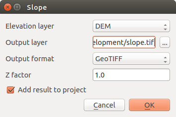
• Set the save location to exercise_data/residential_development/slope.tif

• Enable the Load into canvas... checkbox.

• Click OK and close the dialogs when processing is complete, and click Close to close the dialog. You’ll see a new raster loaded into your map.

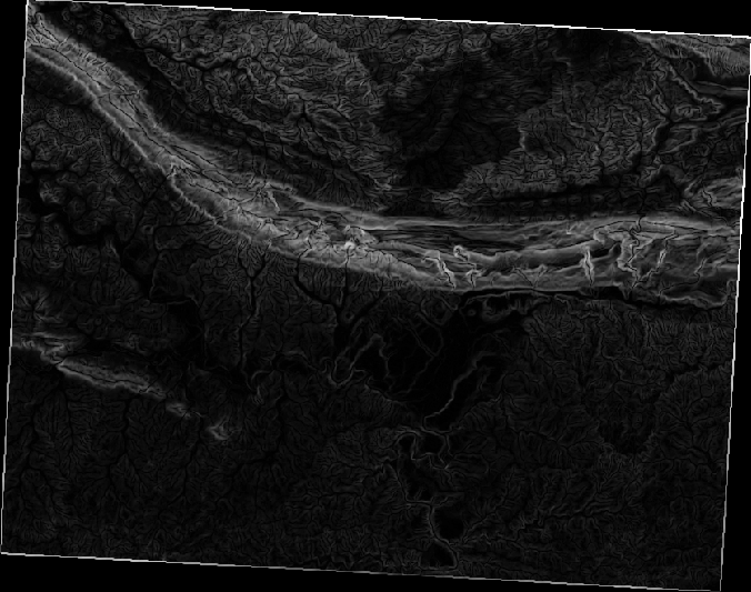
• With the new raster selected in the Layers list, click the Stretch Histogram to Full Dataset button. Now you’ll see the slope of the terrain, with black pixels being flat terrain and white pixels, steep terrain:

  

8.3.4. Try Yourself calculating the aspect¶

The aspect of terrain refers to the direction it’s facing in. Since this study is taking place in the Southern Hemisphere, properties should ideally be built on a north-facing slope so that they can remain in the sunlight.

• Use the Aspect mode of the DEM (Terain models) tool to calculate the aspect of the terrain.

Vérifiez vos résultats

8.3.5. Follow Along: Utilisation de la Calculatrice Raster¶

Rappelez-vous le problème de l’agent immobilier que nous nous sommes posés dans la leçon Analyse Vectorielle. Imaginons que les acheteurs souhaitent maintenant acheter un immeuble et construire un plus petit cottage sur la propriété. Dans l’Hémisphère Sud, nous savons qu’une parcelle idéale pour le développement a besoin d’avoir des zones orientées vers le Nord, et avec une pente de moins de cinq degrés. Mais si la pente est inférieure à 2 degrés, alors l’aspect ne fonctionnera pas.

Heureusement, vous avez déjà des rasters qui vous montrent la pente aussi bien que l’aspect, mais vous n’avez aucune façon de savoir où les deux conditions sont immédiatement satisfaites. Comment cette analyse peut-elle être faite ?

La réponse réside dans la Calculatrice Raster.

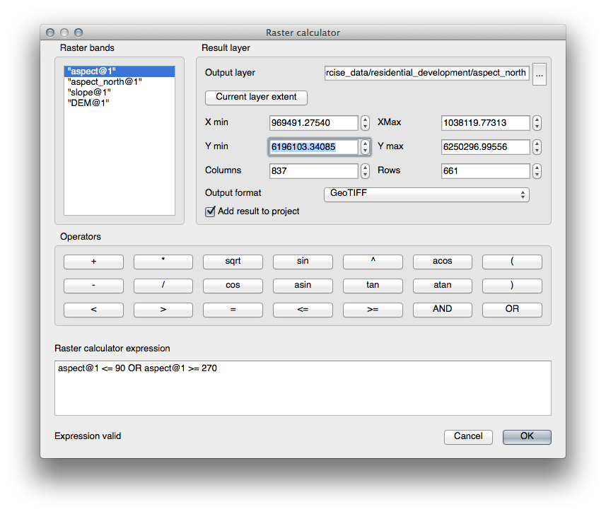
• Click on Raster > Raster calculator... to start this tool.
• To make use of the aspect dataset, double-click on the item aspect@1 in the Raster bands list on the left. It will appear in the Raster calculator expression text field below.

North is at 0 (zero) degrees, so for the terrain to face north, its aspect needs to be greater than 270 degrees and less than 90 degrees.

• In the Raster calculator expression field, enter this expression:

  aspect@1 <= 90 OR aspect@1 >= 270

• Set the output file to aspect_north.tif in the directory exercise_data/residential_development/.

• Ensure that the box Add result to project is checked.

• Click OK to begin processing.

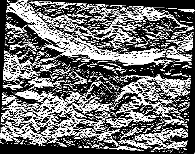
Votre résultat doit être cela :

8.3.6. Try Yourself¶

Maintenant que vous avez fait l’aspect, créez deux nouvelles analyses séparées pour la couche MNE.

• The first will be to identify all areas where the slope is less than or equal to 2 degrees.
• The second is similar, but the slope should be less than or equal to 5 degrees.
• Save them under exercise_data/residential_development/ as slope_lte2.tif and slope_lte5.tif.

Vérifiez vos résultats

8.3.7. Follow Along: Combinaison des résultats de l’analyse raster¶

Vous avez maintenant trois nouvelles analyses raster sur la couche MNE :

• guilabel:aspect_north : le terrain face au nord

• slope_lte2 : la pente inférieure ou égale à 2 degrés

• slope_lte5 : la pente inférieure ou égale à 5 degrés

Where the conditions of these layers are met, they are equal to 1. Elsewhere, they are equal to 0. Therefore, if you multiply one of these rasters by another one, you will get the areas where both of them are equal to 1.

Les conditions à remplir sont : égal ou inférieur à 5 degrés de pente, le terrain doit être orienté au Nord ; mais égal ou inférieur à 2 degrés de pente, la direction vers laquelle le terrain est orienté n’a pas d’importance.

Therefore, you need to find areas where the slope is at or below 5 degrees AND the terrain is facing north; OR the slope is at or below 2 degrees. Such terrain would be suitable for development.

Pour calculer les zones qui satisfont ces critères :

• Open your Raster calculator again.

• Use the Raster bands list, the Operators buttons, and your keyboard to build this expression in the Raster calculator expression text area:

  ( aspect_north@1 = 1 AND slope_lte5@1 = 1 )  OR slope_lte2@1 = 1

• Save the output under exercise_data/residential_development/ as all_conditions.tif.

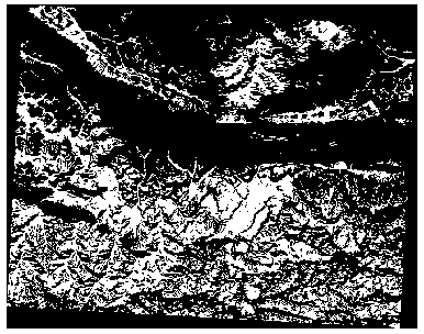
• Click OK on the Raster calculator. Your results:

  

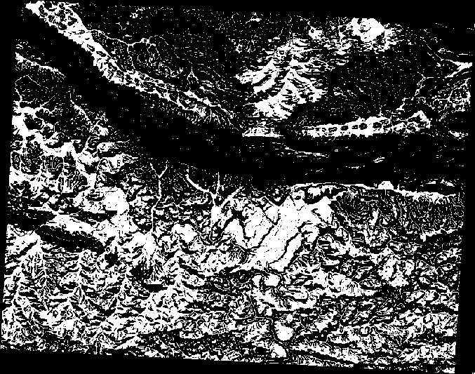
8.3.8. Follow Along: Simplification du Raster¶

Comme vous pouvez le voir dans l’image du bas, l’analyse combinée nous a laissé avec beaucoup de très petites zones où les conditions sont remplies. Mais elles ne sont pas très utiles pour nos analyses, puisqu’elles sont trop petites pour y construire quelque chose. Éliminons toutes ces toutes petites zones inutiles.

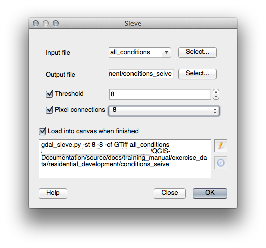
• Open the Sieve tool (Raster ‣ Analysis ‣ Sieve).
• Set the Input file to all_conditions, and the Output file to all_conditions_sieve.tif (under exercise_data/residential_development/).
• Set both the Threshold and Pixel connections values to 8, then run the tool.

Once processing is done, the new layer will load into the canvas. But when you try to use the histogram stretch tool to view the data, this happens:

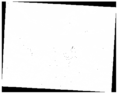
Que se passe-t-il ? La réponse réside dans les fichiers de métadonnées du nouveau raster.

• View the metadata under the Metadata tab of the Layer Properties dialog. Look in the Properties section at the bottom.

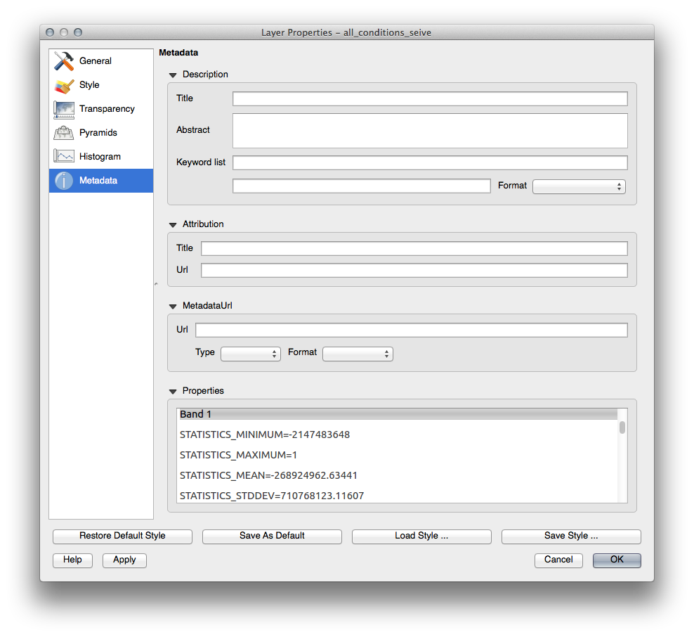
Whereas this raster, like the one it’s derived from, should only feature the values 1 and 0, it has the STATISTICS_MINIMUM value of a very large negative number. Investigation of the data shows that this number acts as a null value. Since we’re only after areas that weren’t filtered out, let’s set these null values to zero.

• Open the Raster Calculator again, and build this expression:

  (all_conditions_sieve@1 <= 0) = 0

  This will maintain all existing zero values, while also setting the negative numbers to zero; which will leave all the areas with value 1 intact.

• Save the output under exercise_data/residential_development/ as all_conditions_simple.tif.

Votre sortie ressemble à cela :

C’est ce qui était attendu : une version simplifiée des résultats précédents. Souvenez-vous que si les résultats que vous obtenez à partir d’un outil ne sont pas ceux que vous attendiez, visualiser les métadonnées (et les attributs vectoriels, si applicable) peut s’avérer essentiel pour résoudre le problème.

8.3.9. In Conclusion¶

You’ve seen how to derive all kinds of analysis products from a DEM. These include hillshade, slope and aspect calculations. You’ve also seen how to use the raster calculator to further analyze and combine these results.

8.3.10. What’s Next?¶

Maintenant que vous avez deux analyse : l’analyse vectorielle qui vous montre les parcelles susceptibles de convenir, et l’analyse raster qui vont montre le terrain susceptibles de convenir. Comment peut-on les combiner pour arriver à un résultat final pour ce problème ? C’est le sujet de la prochaine leçon, qui commence dans le module suivant.